Estimate g(0) and ESW with Auxillary Data

A. Process Previous Survey DAS Data

We are using a broader dataset of false killer whale encounters and associated effort to estimate detectability parameters, g(0) and ESW.

library(tidyverse)
library(Distance)
library(lubridate)
library(here)
library(swfscDAS)
library(MASS)
library(mvnfast)
library(sf)
library(picMaps)

localwd <- here("_R_code","task_2_est_g0_esw")
sp.code <- "033"

Read in previous survey data

#read in input files
das_file <- file.path(localwd, "AllSurveys_g0_ESW_1986-2023.das")
y.proc <- swfscDAS::das_process(das_file)
strata_file_dir <- file.path(localwd, "Strata Files", "region_filter_esw_g0.csv")

Process DAS file and filter for false killer whale regions

y.eff <- swfscDAS::das_effort(
  y.proc, method = "equallength",
  seg.km = 10,
  dist.method = "greatcircle",
  num.cores = 1,
  strata_files = strata_file_dir)
y.eff.sight <- swfscDAS::das_effort_sight(y.eff, sp.codes = sp.code, sp.events = "S")
y.eff.sight.strata <- swfscDAS::das_intersects_strata(y.eff.sight, list(InPoly = strata_file_dir)) 

Export data for use in g(0) and ESW estimation

input_dat<-list()
input_dat$esw.dat <- y.eff.sight.strata$sightinfo %>% 
  filter(SpCode == sp.code, InPoly == 1, OnEffort == TRUE)
input_dat$g0.dat <- y.eff.sight.strata$segdata %>% filter(InPoly == 1, EffType == "S")

saveRDS(input_dat, file.path(localwd, "output","esw_g0_input.rds"))

B. Estimate ESW and g(0) Relative to Beaufort Sea State

If you are not continuing from step A in the same session, the following code must be executed to load the appropriate packages and processed data from step A. Otherwise, this code chunk can be skipped.

#' load packages
library(tidyverse)
library(Distance)
library(lubridate)
library(here)
library(mvnfast)
library(picMaps)
library(future)
library(doFuture)

localwd <- here("_R_code","task_2_est_g0_esw")
sp.code <- "033"


#' Recall saved data from step 1
input_dat <- readRDS(file.path(localwd, "output","esw_g0_input.rds"))

Estimate ESW relative to Beaufort sea state

Here we are using the distance package to fit a half-normal detection function, defined as: \[ p_i(x|\boldsymbol{\theta}_d) = \exp(-x/2\sigma_i^2) \] where the detection range parameter is a function of the Beaufort sea state, \(b_i\), on survey segment \(i\), \[ \log \sigma_i = \theta_{d,0} + \theta_{d,b} b_i. \]

df <- data.frame(distance = input_dat$esw.dat$PerpDistKm, beaufort = input_dat$esw.dat$Bft)
df <- df[complete.cases(df),] 

detfun <- ds(df, formula = ~beaufort, truncation = 5.5, key="hn") 

Model contains covariate term(s): no adjustment terms will be included.

Fitting half-normal key function

AIC= 382.087

No survey area information supplied, only estimating detection function.

summary(detfun)

Summary for distance analysis 
Number of observations :  132 
Distance range         :  0  -  5.5 

Model       : Half-normal key function 
AIC         :  382.087 
Optimisation:  mrds (nlminb) 

Detection function parameters
Scale coefficient(s):  
              estimate         se
(Intercept)  1.2486795 0.22333973
beaufort    -0.1320774 0.05168352

                       Estimate          SE         CV
Average p             0.4805914  0.02942133 0.06121901
N in covered region 274.6616170 24.21359682 0.08815792

plot(detfun, showpoints = TRUE)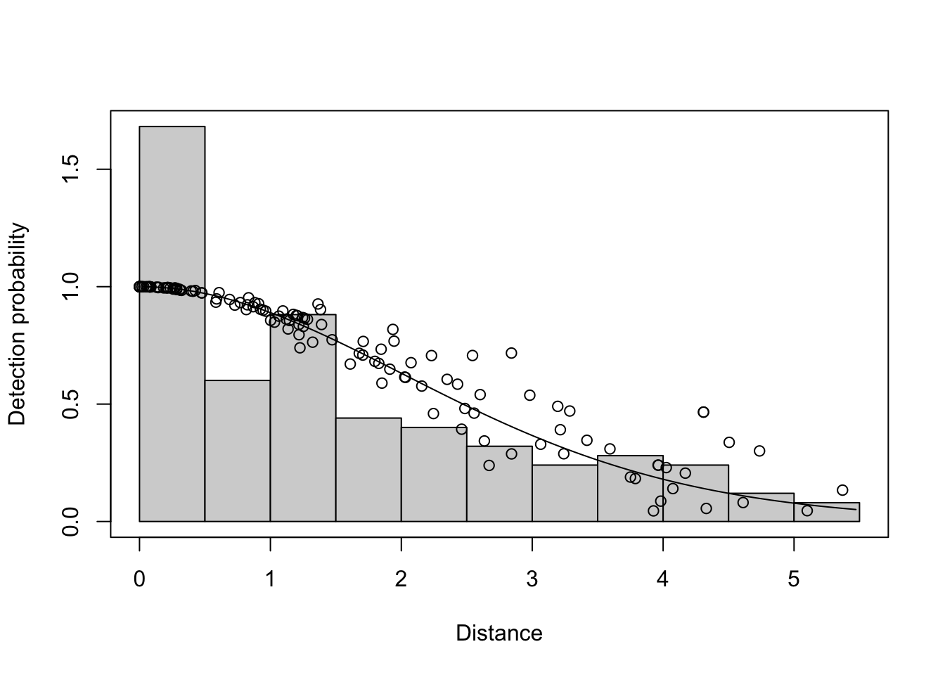

Estimate ESW for all segments

In this step, the effective strip width (\(ESW_i\)) is calculated for each survey segment, \[ ESW_i = \int_0^wp_i(x|\boldsymbol{\theta}_d)dx \] where \(w\) is the truncation width of the transects (here it is 5.5 km as can be seen in the previous code). The \(ESW\) is the width of the strip that would result from a survey with perfect detection. Now the fitted \(ESW\) are saved for future if the user is not continuing on to estimate \(g(0;b_i)\), the probability of detection on the trackline when Beaufort sea state equals \(b_i\).

modeling_data <- readRDS(file.path(here(), "_R_code", "task_1_segment_das_data", "output","seg_sight_out.rds"))
modeling_data$segdata <- modeling_data$segdata %>% rename(beaufort = avgBft)
modeling_data$segdata[paste0("esw","_",sp.code)] <- predict(detfun, modeling_data$segdata, esw=TRUE)[["fitted"]]

Estimate g(0) relative to Beaufort sea state

Now we can use the \(ESW\) results to fit a very general DSM model over false killer whale detections. The density model includes a Beaufort sea state effect so we can assess the relative density of detections in different sea states. By assuming that detection along the trackline is \(g(0;b)=1\) for \(b = 0\) or \(1\) (the calmest seas), we can estimate trackline detection probability during false killer whale surveys. For the DSM model, we need to add the effective survey area, \[ ESA_i = 2 \times ESW_i \times L_i \]where \(L_i\) is the length of segment \(i\). \(ESA_i\) is then used to assess the observed density, \(y_i\) of false killer whales for each segment. Then a GAM is fitted to the observed densities with log expected value: \[ \log E(y_i) = \log ESA_i + f(b_i) + f(Lon_i,Lat_i) + f(year_i) \] where the \(f(\dots)\) terms are nonparametric function effects. To enforce the conditions that \(f(b)\) should be monotonically decreasing as sea state increases, the scam package is used instead of mgcv. When the smooth formulation bs='mpd' is used, this monotonicity is enforced.

g0_dat <- input_dat$g0.dat
g0_dat$resp <- as.logical(g0_dat[,paste0("nSI_",sp.code)])
g0_dat <- g0_dat%>%dplyr::select(resp, mlat, mlon, avgBft, year,dist) %>% 
  rename(beaufort = avgBft)
g0_dat <- g0_dat[complete.cases(g0_dat), ]

g0_dat$esa <- predict(detfun, newdata = g0_dat, esw=TRUE)[["fitted"]] * 2 * g0_dat$dist #predict an ESW for each segment for use in g0 model
g0_dat <- filter(g0_dat, esa>0)

#' Combine beaufort=0,1 as the same g(0) = 1
g0_est<-scam::scam(formula = resp ~ s(I(pmax(beaufort-1,0)), bs='mpd', k=4)
                     + s(mlat, mlon, bs='tp') + s(year, k=4), 
                   offset = log(esa+0.0001),
                   family=poisson,
                   data=g0_dat,
                   not.exp=TRUE,
                   gamma=1.4)

Estimate relative g(0) for each Beaufort sea state

Now that the model is fit, we can estimate \(g(0;b)\) by examining the relative expected density for any specific segment under different Beaufort conditions. Because the \(f(b_i)\) term is additive, it does not matter which is used because they will all be the same. So, we just formulate a generic segment with varying Beaufort states. For the predicted density, \[ \mu_b = E(y_*) = \exp( \log ESA_* + f(b) + f(Lon_*,Lat_*) + f(year_*)), \] the estimated trackline probability is \[ g(0;b) = \mu_b / \mu_0 \]

newdata_g0 <- data.frame(beaufort = 0:7,
                         mlat = mean(modeling_data$segdata$mlat, na.rm=TRUE),
                         mlon = mean(modeling_data$segdata$mlon, na.rm=TRUE),
                         year = round(mean(modeling_data$segdata$year, na.rm=TRUE)))

ps <- scam::predict.scam(g0_est, newdata = newdata_g0, type="response")
Rg0 <- ps/ps[1]
names(Rg0) <- 0:7
round(Rg0,2) # for display only

   0    1    2    3    4    5    6    7 
1.00 1.00 0.70 0.49 0.34 0.23 0.16 0.11 

Add g(0) estimate to all segments and save final modeling data set

To account for survey segments with non-integer Beaufort states, because it changed over the course of the segment, the \(g(0;b)\) value was linearly interpolated between the adjacent \(b\) values. Then model data for the current survey is exported for use in the pelagic false killer whale DSM. The \(g(0;b_i)\) and \(ESW_i\) will serve as an effort offset.

BFlow <- floor(modeling_data$segdata$beaufort + 1)
BFhigh <- ceiling(modeling_data$segdata$beaufort + 1)
w <- BFhigh - (modeling_data$segdata$beaufort + 1)
modeling_data$segdata[,paste0("g0_w_",sp.code)] <- w
modeling_data$segdata[,paste0("g0","_",sp.code)] <- w*Rg0[BFlow] + (1-w)*Rg0[BFhigh]

saveRDS(modeling_data, file.path(localwd, "output","seg_sight_out_g0_ESW.rds"))

C. Monte Carlo Estimation of ESW and g(0) Parameter Covariance Matrix

To propagate the uncertainty for effort terms into the false killer whale DSM model, the covariance matrix for the detection terms needs to be estimated because the \(g(0;b)\) model depends on the \(ESA_i\) values calculated from the distance model. Therefore, the most straightforward method to account for the covariance between the distance sampling parameters, \(\theta_d\) and the \(g(0,b)\) parameters, \(\theta_g\), is to perform a Monte Carlo simulation. First, we sample 5,000 \(\theta_d\) replications from its large sample distribution, \(N(\hat{\theta}_d, V_d)\), where \(\hat{\theta}_d\) are the estimated distance function parameters and \(V_d\) is the estimated covariance matrix. For each replication, we calculate \(ESA_i\) for the survey segments and fit the scam model to estimate the \(f(b)\) parameters, \(\theta_g\). The full estimated covariance matrix, \(V_\theta\), for = \(\hat{\theta}=(\hat{\theta}_d, \hat{\theta}_g)\), was estimated with the empirical covariance matrix of the 5,000 samples.

Warning!!! The following Monte Carlo code takes a very long time to run for the false killer whale analysis. To improve speed of the simulation, we have looped over blocks of smaller simulation in parallel. For the code below we use npar <- 10 separate R instances, each sampling samps <- 500 \(\theta\) values for a total of 5,000 \(\theta\) replications. If you want to see the code in action, we suggest that you dramatically reduce the overall sample size to assess how long it will take the full sample to execute.

# Design matrix for g(0) estimates 
Lp <- scam::predict.scam(g0_est, newdata = newdata_g0, type="lpmatrix")
# Subset for columns affecting g(0):
bft_idx <- grep("beaufort", colnames(Lp))
Lp <- Lp[,bft_idx]

# Draw detection parameter sample:
detfun_g0 <- detfun
v_theta <- solve(detfun_g0$ddf$hessian)
pars.esw <- detfun_g0$ddf$par

npar <- 10
samps <- 500 # total samples = npar * samps

plan("multisession", workers=npar)
set.seed(8675309)

g0_par_sim <- foreach(i = 1:npar,  .options.future = list(seed = TRUE), .errorhandling = "pass") %dofuture% {
  theta_star <- matrix(NA, samps, length(detfun$ddf$par))
  v_alpha_star <- matrix(NA, samps, length(bft_idx)^2)
  alpha_star <- matrix(NA, samps, length(bft_idx))
  Rg0_star <- matrix(NA, samps, 8)
  # Constructing variance-covariance matrix 
  for(j in 1:samps){
    g0_star_out <- sim_esw_g0(pars.esw, v_theta, detfun, g0_dat)
    g0_star <- g0_star_out$g0_star
    theta_star[j,] <-  g0_star_out$theta_star
    v_alpha_star[j,] <- as.vector(g0_star$Vp.t[bft_idx, bft_idx])
    alpha_star[j,] <- g0_star$coefficients.t[bft_idx]
    Rg0_star[j,] <- g0_star_out$Rg0
    
  }
  list(theta_star=theta_star, alpha_star=alpha_star, v_alpha_star=v_alpha_star, Rg0_star=Rg0_star)
}
plan("sequential")

Here, we are combining the parallel samples back together and calculating the covariance matrix \(V_\theta\). Then, we export the results for use in the abundance prediction uncertainty assessment stage.

theta_star <- lapply(g0_par_sim, \(x) x$theta_star) %>% do.call(rbind,.)
alpha_star <- lapply(g0_par_sim, \(x) x$alpha_star) %>% do.call(rbind,.)
v_alpha_star <- lapply(g0_par_sim, \(x) x$v_alpha_star) %>% do.call(rbind,.)
Rg0_star <- lapply(g0_par_sim, \(x) x$Rg0_star) %>% do.call(rbind,.)

## Compose full variance/covariance from law of total variance
v_alpha <- colMeans(v_alpha_star) %>% matrix(.,sqrt(length(.))) +
  var(alpha_star)
c_alpha_theta <- cov(alpha_star, theta_star)
V <- rbind(
  cbind(v_alpha, c_alpha_theta),
  cbind(t(c_alpha_theta), var(theta_star))
)

varprop_list <- list(
  newdata_g0 = newdata_g0,
  Lp_g0 = Lp,
  V_par = V,
  par_sim = cbind(alpha_star, theta_star),
  Rg0_sim = Rg0_star,
  detfun = detfun, 
  g0_dat = g0_dat,
  g0_est = g0_est,
  bft_idx = bft_idx
)

saveRDS(varprop_list, file = file.path(datadir, "output","varprop_list.rds"))