install.packages('dsmextraLite',
repos=c('https://pifsc-protected-species-division.r-universe.dev',
        'https://cloud.r-project.org')
)Assessing Areas of Extrapolation
Note!!! Here we use the methods within the dsmextra package to examine spatial areas of extrapolation. However, at the time this code was written, the dsmextra package was not functioning due to recent changes in the R spatial data ecosystem. The dsmextra package was updated after this analysis. In the future we will investigate including it into the workflow. For this analysis, we pulled the necessary components from the old package and repackaged them as dsmextraLite, available for download and installation with the code snippet:
Packages and preparation
library(terra)
library(tidyverse)
library(foreach)
library(doFuture)
library(ggplot2)
library(ggspatial)
library(tidyterra)
library(picMaps)
library(viridis)
library(here)
library(sf)
library(ggpubr)

library(dsmextraLite)
Load ocean data and segment data
local_wd <- here("_R_code","task_6_examine_extrapolation")
ocean_dir <- here("_R_code","task_5_download_prediction_data","output")
load(here("_R_code","task_4_fit_dsm_models","output","dsm_fit_final.RData"))
ocean_files <- paste(ocean_dir,list.files(ocean_dir), sep="/")
Examine extrapolation regions with dsmExtraLite
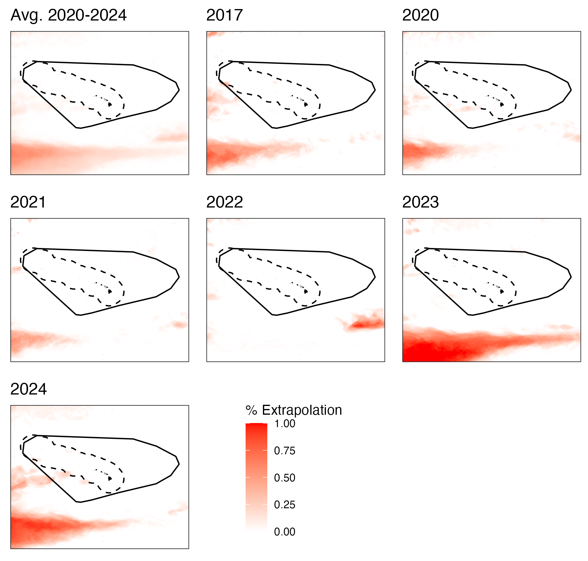
For every day in the prediction data set, we used dsmextraLite to determine if the oceanographic variables in that cell were outside the values that were used to fit the model. For each year and grid cell, we summarized the proportion of the prediction days that were classified as either univariate or combinatorial extrapolation conditions.
fkw_dsm_data <- st_as_sf(fkw_dsm_data, coords=c("mlon","mlat"), crs=4326) %>%
  st_shift_longitude()

# extrapolation <- vector("list",length(ocean_files))

plan("multisession", workers=length(ocean_files))

extrapolation <- foreach(
  i = seq_along(ocean_files),
  .options.future = list(seed = TRUE)
) %dofuture% {
  ocean <- rast(ocean_files[i])
  dates_i <- time(ocean) %>% unique()
  extrap_i <- NULL
  for(j in seq_along(dates_i)){
    ocean_j <- ocean[[time(ocean)==dates_i[j]]]
    extrap_j <- compute_extrapolation(
      samples = fkw_dsm_data,
      covariate.names = c("sst","mld","ssh"),
      prediction.grid = ocean_j
    )
    extrap_i <- c(extrap_i, 1.0*(ifel(!is.na(extrap_j$rasters$ExDet$univariate), 1, 0) | ifel(!is.na(extrap_j$rasters$ExDet$combinatorial), 1, 0)))
  }
  extrap_i <- do.call(c, extrap_i)
  time(extrap_i) <- dates_i
  extrap_i <- wrap(extrap_i)
  extrap_i
}
plan("sequential")

extrapolation <- lapply(extrapolation, unwrap)
extrapolation <- do.call(c, extrapolation)
writeRaster(extrapolation, file=file.path(local_wd, "output", "extrapolation.tif"))
Create figures
hi <- hawaii_coast()
eez <- hawaii_eez()
fkwm <- pfkw_mgmt()
em17 <- extrapolation[[year(time(extrapolation))!=2017]]
e_mean <- mean(em17)
ppp <- vector("list",length(ocean_files)+1)

ppp[[1]] <- ggplot() + geom_spatraster(data=e_mean) +
  layer_spatial(hi, fill="black", color=NA) +
  layer_spatial(eez, color="black", fill=NA, linetype="dashed", lwd=0.5) +
  layer_spatial(fkwm, color="black", fill=NA,lwd=0.5) +
  scale_fill_grass_c("reds",name="% Extrapolation") +
  scale_x_continuous(breaks=c(175, 228)) + scale_y_continuous(breaks=c(0, 40)) +
  theme_bw() + #theme(legend.position="none") +
  theme(axis.text = element_blank(), axis.ticks = element_blank()) +
  coord_sf(expand = FALSE) +
  ggtitle("Avg. 2020-2024")
lll <- get_legend(ppp[[1]])
ppp[[1]] <- ppp[[1]] + theme(legend.position="none")
years <- time(extrapolation) %>% year %>% unique

for(i in seq_along(years)){
  e <- extrapolation[[ year(time(extrapolation))==years[i] ]]
  e <- mean(e)
  ppp[[i+1]] <- ggplot() + geom_spatraster(data=e) +
    layer_spatial(hi, fill="black", color=NA) +
    layer_spatial(eez, color="black", fill=NA, linetype="dashed", lwd=0.5) +
    layer_spatial(fkwm, color="black", fill=NA, lwd=0.5) +
    # scale_fill_viridis(option="H", name="% Extrapolation") +
    # scale_fill_princess_c("maori",name="% Extrapolation") +
    scale_fill_grass_c("reds",name="% Extrapolation") +
    scale_x_continuous(breaks=c(175, 228)) + scale_y_continuous(breaks=c(0, 40)) +
    theme_bw() + theme(legend.position="none") +
    theme(axis.ticks = element_blank()) +
    theme(axis.text = element_blank(), axis.ticks = element_blank()) +
    coord_sf(expand = FALSE) +
    ggtitle(years[i])
}

pout <- ggarrange(ppp[[1]], ppp[[2]], ppp[[3]], ppp[[4]], ppp[[5]], ppp[[6]], ppp[[7]],lll)
ggsave(pout, file=file.path(local_wd, "output","extrap_fig.png"), width=6.5, height=6.2)
Visual extrapolation assessment
Proportion of days each year where grid cells were classified as having extrapolation conditions. Deeper red hues represent more days with extrapolation conditions.