Fit and Select DSMs using GAMs

A. Data Preparation

Load data

Here, we load the survey segment data and sighting data from steps 1 and 2 and clean it up for DSM fitting with the mgcv package.

localwd <- here("_R_code","task_4_fit_dsm_models")

segDataESWg0 <- readRDS( here("_R_code","task_2_est_g0_esw","output","seg_sight_out_g0_ESW.rds") )

#' Read table defining which sightings are from the pelagic population
fkw_popData <- readRDS( here("_R_code", "task_4_fit_dsm_models", "FKWsights_DSM_1997to2023.rds") ) 

spcode <- '033' # FKW code
segDataESWg0$sightinfo <- segDataESWg0$sightinfo %>% filter(SpCode==spcode)%>% #filter for species code
  dplyr::mutate(CruiseSightNo = paste(Cruise,SightNo,sep="-"))%>% 
  filter(CruiseSightNo %in% fkw_popData$CruiseSightNo) #filter for selected sightings 

# Add probability the sighting is of the pelagic stock 
segDataESWg0$sightinfo <- segDataESWg0$sightinfo %>% left_join(.,fkw_popData[,c("CruiseSightNo","ProbPel","EffGrpSizeFull","EffGrpSizePelagic")], by="CruiseSightNo") 
segDataESWg0$sightinfo$nSI_033 <- 1
segDataESWg0$sightinfo$ANI_033 <- segDataESWg0$sightinfo$EffGrpSizeFull

sightinfo <- segDataESWg0$sightinfo %>% select(segnum, ProbPel, nSI_033, ANI_033)

segDataESWg0$segdata <- select(segDataESWg0$segdata, -nSI_033, -ANI_033)
segDataESWg0$segdata <- left_join(segDataESWg0$segdata, sightinfo)
segDataESWg0$segdata <- segDataESWg0$segdata %>% mutate(
  nSI_033 = ifelse(is.na(nSI_033), 0, nSI_033),
  ANI_033 = ifelse(is.na(ANI_033), 0, ANI_033),
  ProbPel = ifelse(is.na(ProbPel), 1, ProbPel)
)

write.csv(segDataESWg0$sightinfo, file.path(localwd, "output", "sightinfo_033.csv" ), row.names = FALSE)

Attach environmental data and save for DSM fitting

Now, we attach the oceanographic data to the model data.

segEnvData <- readRDS(file.path(here(), "_R_code","task_3_download_env_data","output","segdata_env.rds")) %>% 
  select(segnum, Latitude, Longitude, UTC, sst:ssh_sd)
segdata <- left_join(segDataESWg0$segdata, segEnvData, by="segnum")

saveRDS(segdata, file.path(localwd, "output", "fkw_dsm_data_1997to2024.rds") )
write.csv(segdata, file.path(localwd, "output", "fkw_dsm_data_1997to2024.csv"), row.names = FALSE)

B. DSM Formulation and Fitting

Load and add effort calculation to data

local_wd <- file.path(here(), "_R_code", "task_4_fit_dsm_models")
fkw_dsm_data <- readRDS(file.path(local_wd, "output", "fkw_dsm_data_1997to2024.rds"))

#' Add effort data
fkw_dsm_data <- fkw_dsm_data %>% mutate(
  effort = g0_033 * 2 * esw_033 * dist
)

#' Filter out years without any sightings
nz_sight <- fkw_dsm_data %>% group_by(year) %>% summarize(sightings = sum(nSI_033)) %>% 
  filter(sightings>0)

fkw_dsm_data <- fkw_dsm_data %>% filter(year%in%nz_sight$year, beaufort<7, effort>0)
fkw_gs <- fkw_dsm_data %>% filter(nSI_033 > 0)# Just segments with sightings

Add augmented data for pelagic probability weighting

Here, we add the augmented data for mixture-like weighting of encounters where the probability that the sighting is of pelagic false killer whales is less than 1. For all sightings with ProbPel < 1, we add an additional line of data for each segment where the number of groups detected is nSI_033 <- 0 and ProbPel <- 1-ProbPel for the observed encounter.

nonpel <- fkw_dsm_data %>% filter(ProbPel<1)
nonpel <- nonpel %>% mutate(
  nSI_033 = 0,
  ProbPel = 1-ProbPel,
  augment=1
)

fkw_dsm_data <- bind_rows(fkw_dsm_data, nonpel) %>% 
  mutate(
    augment = ifelse(is.na(augment), 0, 1)
  )

Create model list and fit

In this section of code, we construct a list for all desired encounters and groups size model specifications. We then fit all the models and produce a table of models and AIC values.

Encounter rate models

Specification of the encounter rate model set is somewhat tricky due to the fact there are are several restrictions on the set of all possible models, namely due to the inclusion of Latitude interaction effects. The encounter rate models included all combinations of the 4 oceanographic variables: sst, ssh, mld, and salinity (including none) along with all combinations of the focal standard deviation versions: sst_sd, ssh_sd, mld_sd, and salinity_sd. The _sd versions are meant to examine the effect of fronts within the gradients of these variables. In addition to this model set, we also added an interaction term of the form te(var,Latitude) for interaction effects of Latitude on the main variables. Only 1 main variable was allowed to interact with Latitude at a time. The resulting list is comprised of 767 models.

hab_var <- c("sst","ssh","mld","salinity")
hab_var_sd <- c("sst_sd","ssh_sd","mld_sd","salinity_sd")

hab_inc <- expand.grid(rep(list(0:2), length(hab_var)))
hab_inc <- hab_inc[apply(hab_inc==2, 1, sum)<2,]
hab_sd_inc <- expand.grid(rep(list(0:1), length(hab_var_sd)))

form_hab <- apply(hab_inc, 1, function(row) {
  terms <- mapply(function(choice, var) {
    if (choice == 1) return(paste0("s(",var,",bs=spline2use,k=5)"))
    if (choice == 2) return(paste0("te(", var, ",Latitude,bs=spline2use,k=5)"))
    return(NULL)
  }, row, hab_var)
  terms <- unlist(terms)
  if (length(terms) == 0) return("nSI_033 ~ ")  # skip null model
  paste("nSI_033 ~", paste(terms, collapse = " + "))
}) %>% unlist()

form_hab_sd <- apply(hab_sd_inc, 1, function(row) {
  terms <- mapply(function(choice, var) {
    if (choice == 1) return(paste0("s(",var,",bs=spline2use,k=5)"))
    return(NULL)
  }, row, hab_var_sd)
  terms <- unlist(terms)
  # if (length(terms) == 0) return(NULL)  # skip null model
  paste(terms, collapse = " + ")
}) %>% unlist()

forms_er <- NULL
for(i in seq_along(form_hab)){
  if(i ==1) {
    tmp <- paste(form_hab[i], form_hab_sd[-1], sep="")
  } else {
    tmp <- c(form_hab[i], paste(form_hab[i], form_hab_sd[-1], sep=" + "))
  }
  forms_er <- c(forms_er, tmp)
}

Fit all encounter rate models

In this section, we fit all 767 encounter rate models to determine the AIC optimal model, as well as the relative rankings of different models, etc.

Warning!!! This takes a while to implement, so it was partitioned and chunks of models were fit in parallel.

#' Select spline type
#' 'ts'= thin plate splines ("shrinkage approach" applies additional smoothing penalty)
#' "tp" is default for s()
spline2use <- "ts" 

workers <- 8
plan("multisession", workers=workers)
# forms <- split(forms, cut(seq_along(forms), breaks = workers, labels = FALSE))

with_progress({
  pb <- progressor(along = forms_er) 
  ergam_list <- foreach(
    i = seq_along(forms_er), .options.future = list(seed = TRUE), 
    .errorhandling = "pass") %dofuture% {
      spline2use <- spline2use
      gam_fit <- gam(formula = as.formula(forms_er[i]), offset = log(effort),
                     family = tw(),
                     method="REML", 
                     data = fkw_dsm_data, weights = ProbPel)
      pb()
      list(summary = summary(gam_fit), aic=gam_fit$aic)
    }
})
plan("sequential")

mod_df <- data.frame(
  idx = 1:length(ergam_list),
  form = forms_er, 
  aic = sapply(ergam_list, \(x) x$aic), 
  dev_expl=sapply(ergam_list, \(x) x$summary$dev.expl*100)
) %>% mutate(
  waic = exp(-0.5*(aic-min(aic))),
  waic = waic/sum(waic)
) %>% arrange(desc(waic))

Group size model

The group size model set is relatively easy to fit as it simply consists of every combination of the 4 oceanographic variables for a total of 16 models.

hab_inc_gs <- expand.grid(rep(list(0:1), length(hab_var)))
forms_gs <- apply(hab_inc_gs, 1, function(row) {
  terms <- mapply(function(choice, var) {
    if (choice == 1) return(paste0("s(",var,",bs=spline2use,k=5)"))
    return(NULL)
  }, row, hab_var)
  terms <- unlist(terms)
  # if (length(terms) == 0) return(NULL)  # skip null model
  paste(terms, collapse = " + ")
}) %>% unlist()
forms_gs <- paste("log(ANI_033)", forms_gs, sep=" ~ ")
forms_gs[1] <- "log(ANI_033) ~ 1"

Fit all group size models

gsgam_list <- foreach(
  i = seq_along(forms_gs), .options.future = list(seed = TRUE), 
  .errorhandling = "pass") %do% {
    spline2use <- spline2use
    gam_fit <- gam(formula = as.formula(forms_gs[i]),
                   method="REML", 
                   data = fkw_gs, weights = ProbPel)
    list(summary = summary(gam_fit), aic=gam_fit$aic)
  }

mod_df_gs <- data.frame(
  idx = 1:length(gsgam_list),
  form = forms_gs, 
  aic = sapply(gsgam_list, \(x) x$aic), 
  dev_expl=sapply(gsgam_list, \(x) x$summary$dev.expl*100)
) %>% mutate(
  waic = exp(-0.5*(aic-min(aic))),
  waic = waic/sum(waic)
) %>% arrange(desc(waic))

AIC tables

A preview of the resulting AIC results is shown below. The full results are in the exported files "output/aic_er.csv" and "output/aic_gs.csv".

# A tibble: 767 × 6
    ...1   idx form                                         aic dev_expl    waic
   <dbl> <dbl> <chr>                                      <dbl>    <dbl>   <dbl>
 1     1    90 nSI_033 ~ te(sst,Latitude,bs=spline2use,k…  398.     5.93 0.00638
 2     2    91 nSI_033 ~ te(sst,Latitude,bs=spline2use,k…  398.     5.93 0.00638
 3     3   411 nSI_033 ~ te(sst,Latitude,bs=spline2use,k…  398.     5.93 0.00638
 4     4    94 nSI_033 ~ te(sst,Latitude,bs=spline2use,k…  398.     5.93 0.00638
 5     5   218 nSI_033 ~ te(sst,Latitude,bs=spline2use,k…  398.     5.93 0.00638
 6     6   219 nSI_033 ~ te(sst,Latitude,bs=spline2use,k…  398.     5.93 0.00638
 7     7   414 nSI_033 ~ te(sst,Latitude,bs=spline2use,k…  398.     5.93 0.00638
 8     8   410 nSI_033 ~ te(sst,Latitude,bs=spline2use,k…  398.     5.93 0.00638
 9     9    95 nSI_033 ~ te(sst,Latitude,bs=spline2use,k…  398.     5.93 0.00638
10    10   538 nSI_033 ~ te(sst,Latitude,bs=spline2use,k…  398.     5.93 0.00638
# ℹ 757 more rows

# A tibble: 16 × 5
     idx form                                              aic  dev_expl    waic
   <dbl> <chr>                                           <dbl>     <dbl>   <dbl>
 1     7 log(ANI_033) ~ s(ssh,bs=spline2use,k=5) + s(ml…  85.7  2.88e+ 1 2.38e-1
 2     8 log(ANI_033) ~ s(sst,bs=spline2use,k=5) + s(ss…  85.7  2.88e+ 1 2.38e-1
 3    16 log(ANI_033) ~ s(sst,bs=spline2use,k=5) + s(ss…  85.7  2.88e+ 1 2.38e-1
 4    15 log(ANI_033) ~ s(ssh,bs=spline2use,k=5) + s(ml…  85.7  2.88e+ 1 2.38e-1
 5    13 log(ANI_033) ~ s(mld,bs=spline2use,k=5) + s(sa…  92.8  1.24e+ 1 6.81e-3
 6    14 log(ANI_033) ~ s(sst,bs=spline2use,k=5) + s(ml…  92.8  1.24e+ 1 6.81e-3
 7     5 log(ANI_033) ~ s(mld,bs=spline2use,k=5)          92.8  1.23e+ 1 6.81e-3
 8     6 log(ANI_033) ~ s(sst,bs=spline2use,k=5) + s(ml…  92.8  1.23e+ 1 6.81e-3
 9     3 log(ANI_033) ~ s(ssh,bs=spline2use,k=5)          93.6  1.07e+ 1 4.63e-3
10    11 log(ANI_033) ~ s(ssh,bs=spline2use,k=5) + s(sa…  93.6  1.07e+ 1 4.63e-3
11     4 log(ANI_033) ~ s(sst,bs=spline2use,k=5) + s(ss…  93.6  1.07e+ 1 4.63e-3
12    12 log(ANI_033) ~ s(sst,bs=spline2use,k=5) + s(ss…  93.6  1.07e+ 1 4.63e-3
13     1 log(ANI_033) ~ 1                                 96.9 -3.62e-14 8.85e-4
14     9 log(ANI_033) ~ s(salinity,bs=spline2use,k=5)     96.9  1.73e- 3 8.85e-4
15    10 log(ANI_033) ~ s(sst,bs=spline2use,k=5) + s(sa…  96.9  4.62e- 4 8.85e-4
16     2 log(ANI_033) ~ s(sst,bs=spline2use,k=5)          96.9  1.45e- 4 8.85e-4

write.csv(mod_df, file = file.path(local_wd, "output", "aic_er.csv"))
write.csv(mod_df_gs, file = file.path(local_wd, "output", "aic_gs.csv"))
save( fkw_dsm_data, fkw_gs, spline2use, file=file.path(local_wd, "output","dsm_model_data.RData"))

C. Model Evaluation

Load previous AIC results and data

library(mgcv)
library(here)
library(tidyverse)
library(sf)
library(picMaps)
library(units)
library(WeightedROC)
library(gratia)

local_wd <- here("_R_code", "task_4_fit_dsm_models")
load(file.path(local_wd, "output","dsm_model_data.RData"))
aic_er <- read_csv(file.path(local_wd, "output","aic_er.csv"))
aic_gs <- read_csv(file.path(local_wd, "output","aic_gs.csv"))

Fit top models and examine

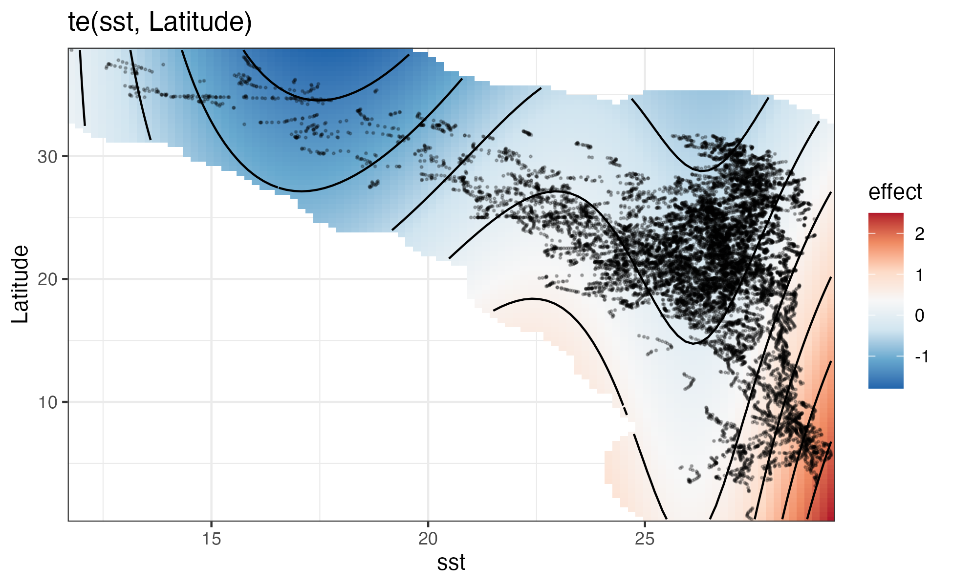
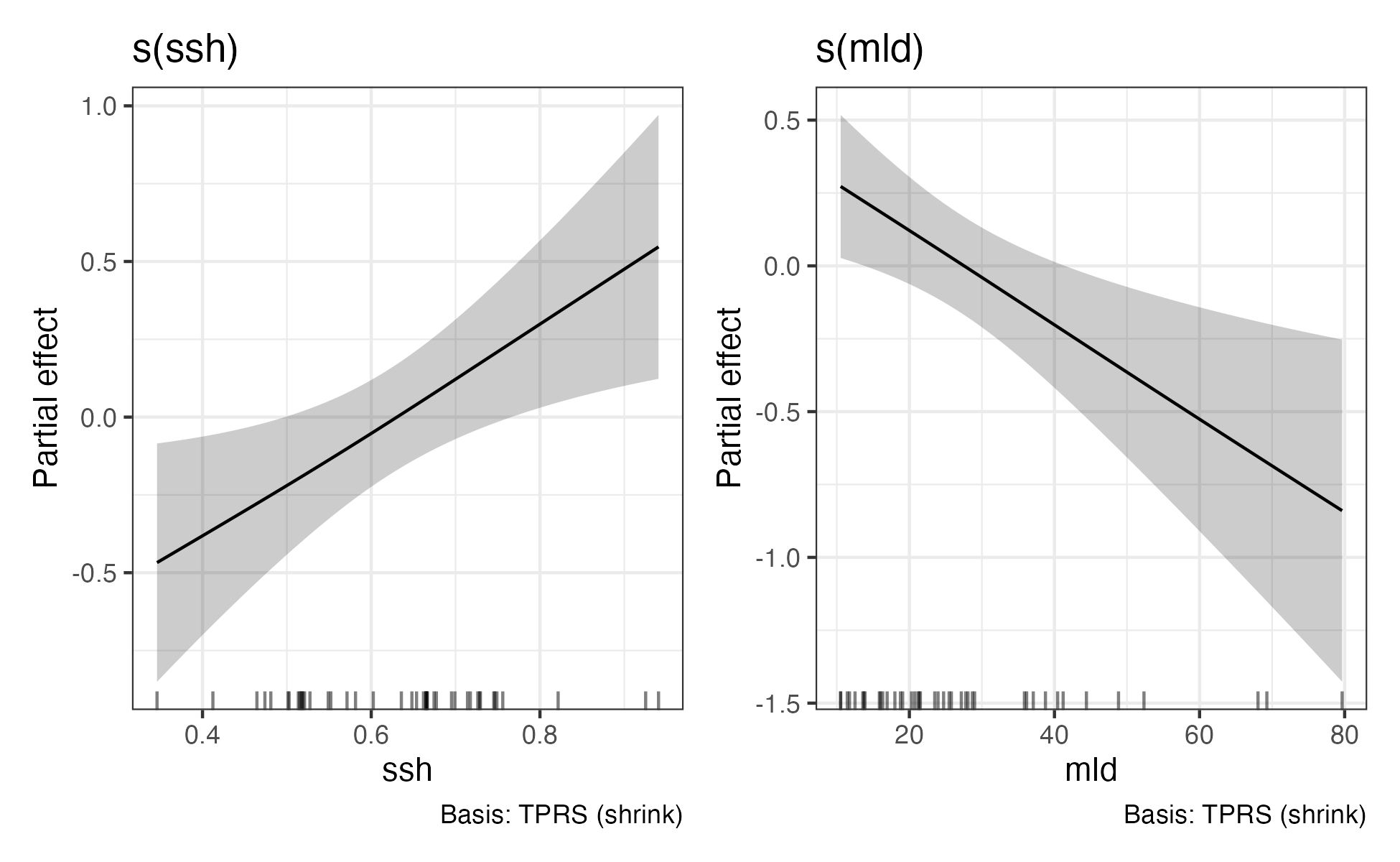
Here, we fit the AIC top models and examine the significance of the effects. For the encounter rate model only, the te(sst, Latitude) effect was statistically significant, so it was retained going forward. For the group size model, all terms were statistically significant, so it is used as is.

# Use top AIC model minus non-significant terms

# er_fit <- gam(formula =as.formula(aic_er$form[1]),
#               offset = log(effort),
#               family = tw(),
#               method="REML", 
#               data = fkw_dsm_data, weights = ProbPel)

er_fit <- gam(formula = nSI_033 ~ te(sst, Latitude, bs = spline2use, k = 5),
              offset = log(effort),
              family = tw(),
              method="REML", 
              data = fkw_dsm_data, weights = ProbPel)
gs_fit <- gam(formula = log(ANI_033) ~ s(ssh, bs = spline2use, k = 5) + s(mld, bs = spline2use, k = 5),
              method="REML", 
              data = fkw_gs, weights = ProbPel)

Evaluate chosen models

Traditional cross-validation is not possible for this analysis due to limited data availability to discretize into training and testing datasets. So, we use other methods of evaluating model performance.

Evaluate ratio of observed to predicted density

Here we examine the ratio of observed to predicted density estimates on the survey segments.

### CenPac area
A <- picMaps::cenpac() %>% st_area() %>% set_units("km^2") %>% as.numeric()

### model predictions
pred_er <- exp(predict(er_fit) + log(fkw_dsm_data$effort))
pred_gs <- exp(predict(gs_fit) + 0.5*gs_fit$sig2)
gs_bias_corr <- weighted.mean(fkw_gs$ANI_033,w=fkw_gs$ProbPel)/mean(pred_gs)
pred_gs <- exp(predict(gs_fit, newdata=fkw_dsm_data) + 0.5*gs_fit$sig2)

### observed
obsdens <- (fkw_dsm_data$nSI_033 * fkw_dsm_data$ANI_033)
ltdens <- weighted.mean(obsdens,fkw_dsm_data$ProbPel)/weighted.mean(fkw_dsm_data$effort,fkw_dsm_data$ProbPel)
ltdens*A
# 23441.83

## predicted
modeldens <- pred_er * pred_gs * gs_bias_corr
preddens <- sum(modeldens)/sum(fkw_dsm_data$effort)
preddens*A
# 22154.7

# Ratio
ltdens/preddens 
# 1.058097

Performance metrics

Standard metrics from `mgcv`

gam.check(er_fit)
qq.gam(er_fit, rep=100, cex=4)

Method: REML   Optimizer: outer newton
full convergence after 18 iterations.
Gradient range [-0.0008121005,5.945633e-05]
(score 200.2306 & scale 1.071581).
Hessian positive definite, eigenvalue range [5.945613e-05,3544.944].
Model rank =  25 / 25 

Basis dimension (k) checking results. Low p-value (k-index<1) may
indicate that k is too low, especially if edf is close to k'.

                    k'   edf k-index p-value
te(sst,Latitude) 24.00  3.76    0.85    0.14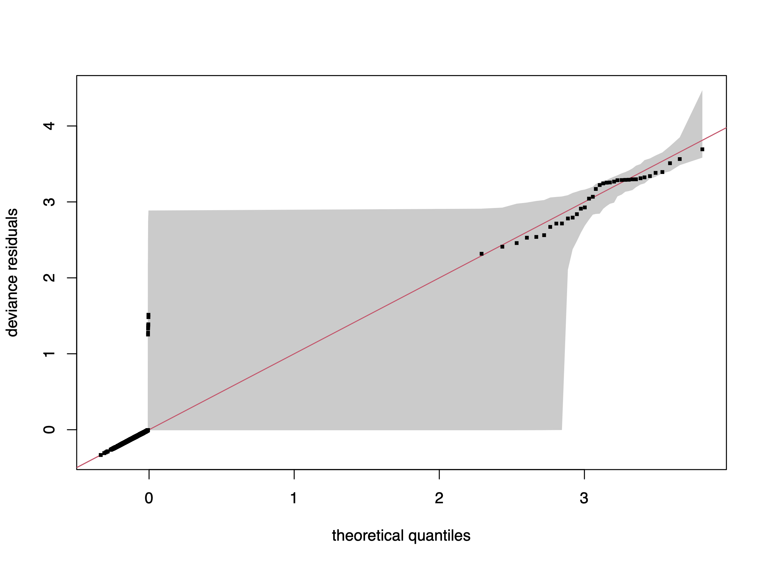

gam.check(gs_fit)
qq.gam(gs_fit, rep=100, cex=4)

Method: REML   Optimizer: outer newton
full convergence after 6 iterations.
Gradient range [-4.679584e-08,3.065578e-08]
(score 43.81738 & scale 0.2549699).
Hessian positive definite, eigenvalue range [0.3710348,21.52089].
Model rank =  9 / 9 

Basis dimension (k) checking results. Low p-value (k-index<1) may
indicate that k is too low, especially if edf is close to k'.

          k'   edf k-index p-value
s(ssh) 4.000 0.952    1.09    0.61
s(mld) 4.000 0.927    1.25    0.93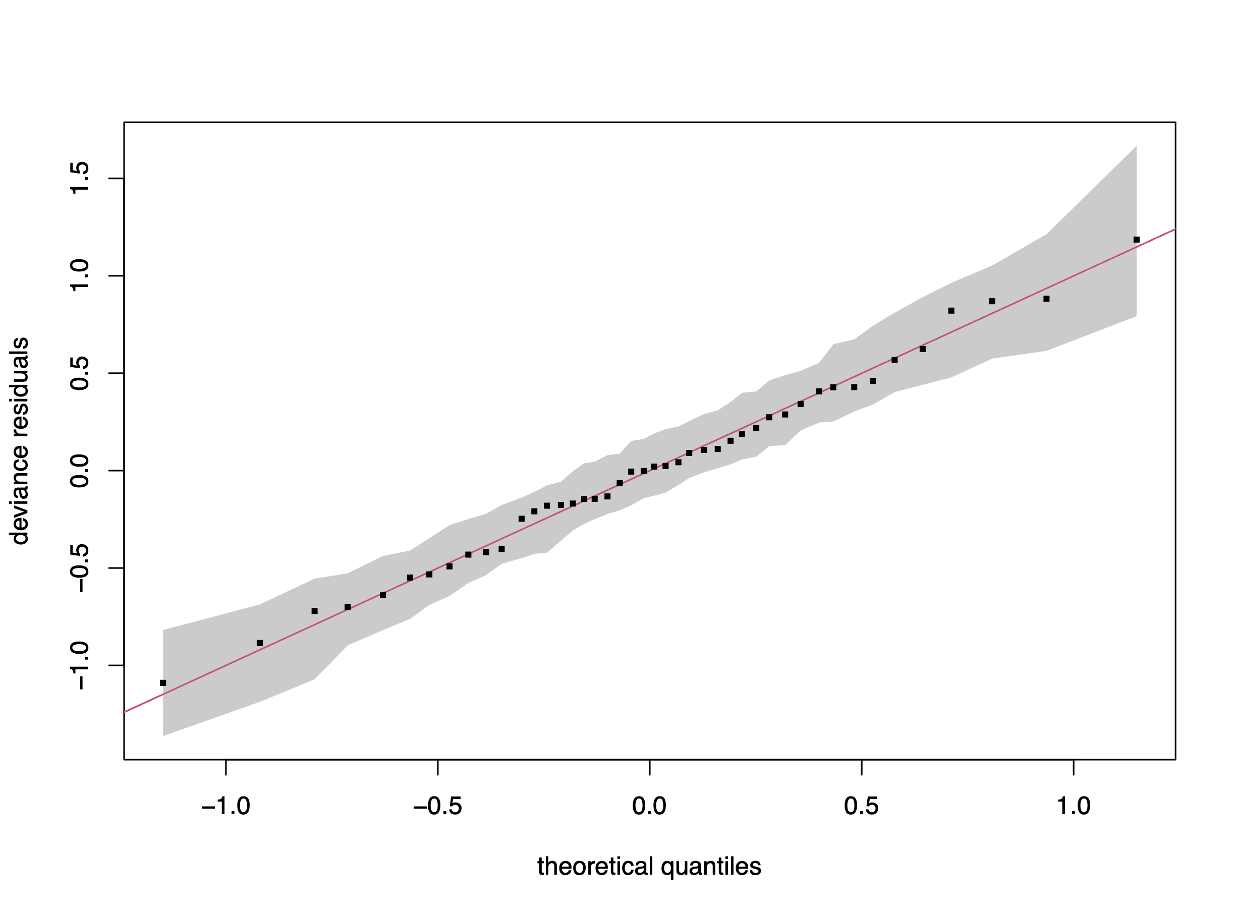

AUC and TSS

Here, we calculate the area under the receiver operating characteristic curve (AUC) and the true skill statistic (TSS). AUC discriminates between true-positive and false-positive rates, and values range from 0 to 1, where a score of > 0.5 indicates better than random discrimination. TSS accounts for both omission and commission errors and ranges from -1 to 1, where 1 indicates perfect agreement and values of zero or less indicate performance no better (or worse) than random.

sightings <- as.numeric(fkw_dsm_data$nSI_033>=1)
pred_seg <- predict(er_fit, type="response") * pred_gs * gs_bias_corr 

rocr <- WeightedROC(pred_seg, sightings, weight = fkw_dsm_data$ProbPel)

## AUC
auc <- WeightedAUC(rocr)
auc
# 0.7119164

## Compute TSS
d <- sqrt((rocr$TPR-1)^2 + (rocr$FPR-0)^2)
which(d==min(d))
opt_rocr <- rocr[which(d==min(d)),]

TSS <- opt_rocr$TPR + (1-opt_rocr$FPR) -1 
TSS
# 0.3626605

ROSE bootstrap sample AUC and TSS

Menardi and Torelli (2014)¹ note that when data are highly imbalanced, performance metrics, such as AUC and TSS, as well as parameter estimation, can be compromised. So, in addition to the AUC and TSS calculations, we also used the ROSE (Random Over-Sampling Examples) sampling bootstrap (Lunardon et al., 2014)² to assess the effects that sparse detection of false killer whales might have had on AUC and TSS metrics for the just the encounter rate model as it is the portion that is severely imbalanced. In the ROSE sampling method, kernel density estimates are calculated for segments with and without detections. Then a sample is drawn with probability = 0.5 from each KDE until the desired sample size is reached. This produces a balanced sample where the predictive covariates are similar to what was observed for each group (detection vs. nondetection) in the original data.

rose_df <- fkw_dsm_data %>% select(
  nSI_033, sst, sst_sd, salinity, salinity_sd, mld, mld_sd, ssh, ssh_sd, Latitude, Longitude, effort
) %>% rename(cls = nSI_033)

auc_stor <- rep(NA, 50)
tss_stor <- rep(NA, 50)
for(i in 1:50){
  resamp <- ROSE(cls~., data=rose_df, hmult.majo=0.25, hmult.mino=0.25, seed=i)$data
  er_fit_rose <- gam(formula = cls ~ te(sst, Latitude, bs = spline2use, k = 5),
                     family = tw(),
                     method="REML", 
                     data = resamp)
  mu <- predict(er_fit_rose, newdata = fkw_dsm_data, type="response")
  phi <- er_fit_rose$sig2
  theta <- er_fit_rose$family$getTheta()
  p <- (1+2*exp(theta))/(1+exp(theta)); p <- max(1.01, p); p <- min(1.99, p)
  pnz <- 1 - exp(- (mu^(2-p)/(phi*(2-p))))
  rrr <-  WeightedROC(pnz, sightings, weight = fkw_dsm_data$ProbPel)
  auc_stor[i] <- WeightedAUC(rrr)
  tss_stor[i] <- max(rrr$TPR + (1-rrr$FPR) -1, na.rm=T)
  cat(i," ")
}
mean(auc_stor)
# 0.7626317
range(auc_stor)
# 0.7581797 0.7666302

mean(tss_stor)
# 0.4331774
range(tss_stor)
# 0.4144445 0.4537293

Examine model effects

sm_grid <- smooth_estimates(er_fit, select = "te(sst,Latitude)")
out <- exclude.too.far(sm_grid$sst, sm_grid$Latitude, fkw_dsm_data$sst, fkw_dsm_data$Latitude, 0.1)
sm_grid$.estimate[out] <- NA
ggplot(data = sm_grid) +
  geom_raster(aes(x = sst, y = Latitude, fill = .estimate)) +
  geom_contour(aes(x = sst, y = Latitude, z = .estimate), colour = "black") +
  geom_point(
    data = dat_res,
    aes(x = sst, y = Latitude),
    size = 0.25, 
    alpha = 0.25 
  ) +
  labs(title = "te(sst, Latitude)") + 
  scale_fill_distiller(palette = "RdBu", type = "div", name = "effect", na.value = NA) +
  coord_cartesian(expand = FALSE) +  theme_bw()
ggsave(file=file.path(local_wd,"output","er_fit.png"),width=6.5, height=4)

draw(gs_fit) & theme_bw()
ggsave(file=file.path(local_wd,"output","gs_fit.png"),width=6.5, height=4)

save(er_fit, gs_fit, gs_bias_corr, opt_rocr, fkw_dsm_data, fkw_gs, A, ltdens, spline2use,
     file=file.path(local_wd, "output", "dsm_fit_final.RData"))

Encounter rate model

Group size model

Footnotes

Menardi, G., and Torelli, N., 2014. Training and assessing classification rules with imbalanced data. Data Mining and Knowledge Discovery, 28:92–122. doi:10.1007/s10618-012-0295-5.↩︎
Lunardon, N., Menardi, G. and Torelli, N. 2014. ROSE: a package for binary imbalanced learning. The R Journal, 6:79–89. doi:10.32614/RJ-2014-008.↩︎

A. Data Preparation

Load data

Attach environmental data and save for DSM fitting

B. DSM Formulation and Fitting

Load and add effort calculation to data

Add augmented data for pelagic probability weighting

Create model list and fit

Encounter rate models

Fit all encounter rate models

Group size model

Fit all group size models

AIC tables

C. Model Evaluation

Load previous AIC results and data

Fit top models and examine

Evaluate chosen models

Evaluate ratio of observed to predicted density

Performance metrics

Standard metrics from mgcv

AUC and TSS

ROSE bootstrap sample AUC and TSS

Examine model effects

Encounter rate model

Group size model

Footnotes

Standard metrics from `mgcv`