Chapter 12 Diagnostic plots
To demonstrate how LTA results can explored quickly and reviewed for QA/QC using diagnostic plots, we will use a built-in LTabundR dataset, which has density/abundance estimates for the Hawaiian EEZ in 2010 and 2017 for striped dolphins, Fraser’s dolphins, and melon-headed whales, ran with only 100 iterations:
We created these LTA results using the following built-in processed dataset:
The function lta_diagnostics() can be used to review the object returned by the LTabundR function lta(), which is the primary function in this package for line-transect analysis. The typical way to use this function is simply:
When you run this, the function will step through many diagnostic outputs (there are currently 8), some of which are tables and some of which are plots. Between each output, the function will wait for the user to press <Enter>. To turn that waiting feature off, you can add the input wait = FALSE.
To see which outputs are currently available from this function, use the following code:
lta_diagnostics(lta_result,
options = c(),
describe_options = TRUE)
List of options for outputs to provide: ===============
(use numbers in the input `options`)
1 - Point estimate (encounter rate, density, abundance, g(0), etc.)
2 - Summary of bootstrap iterations, including CV of density/abundance
3 - Plot of detection function
4 - Histogram of bootstrapped detection counts
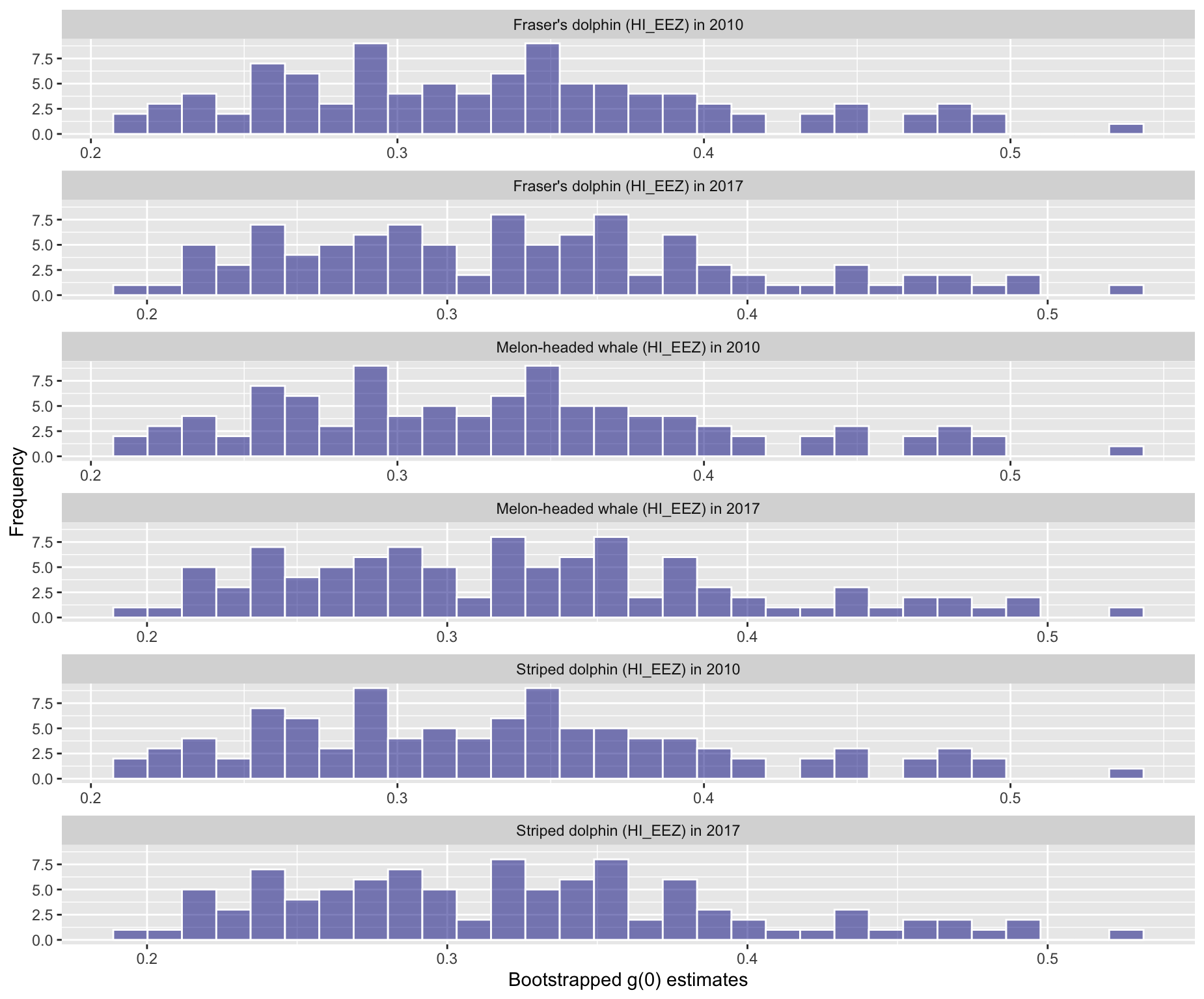
5 - Histogram of bootstrapped g(0) values
6 - Histogram of bootstrapped abundance estimates
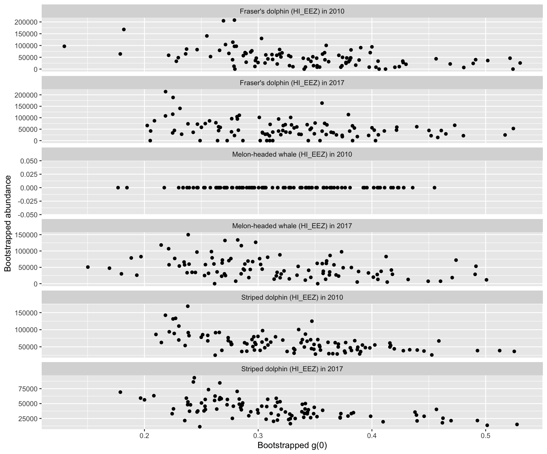
7 - Scatterplot of abundance ~ g(0) relationship in boostraps
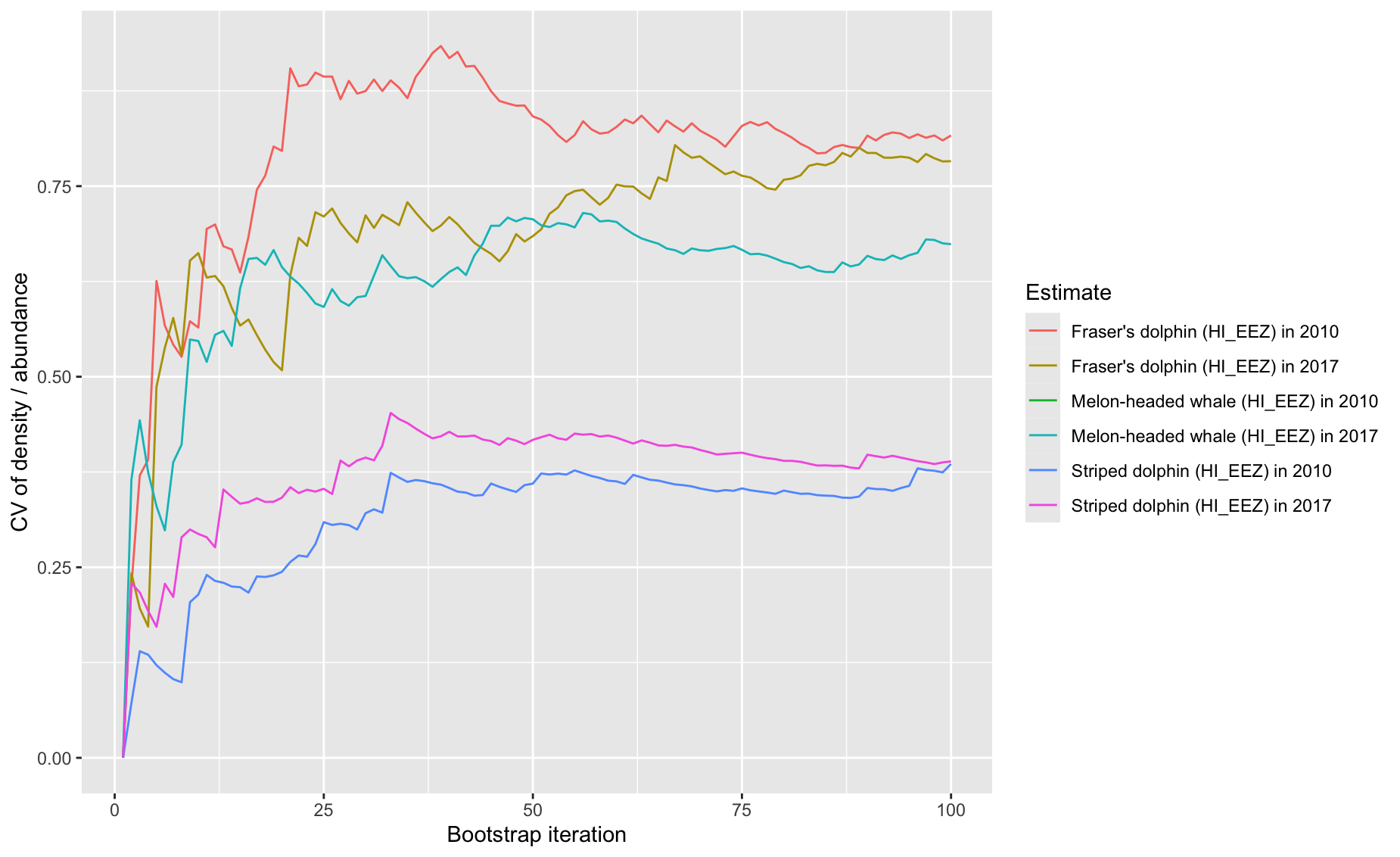
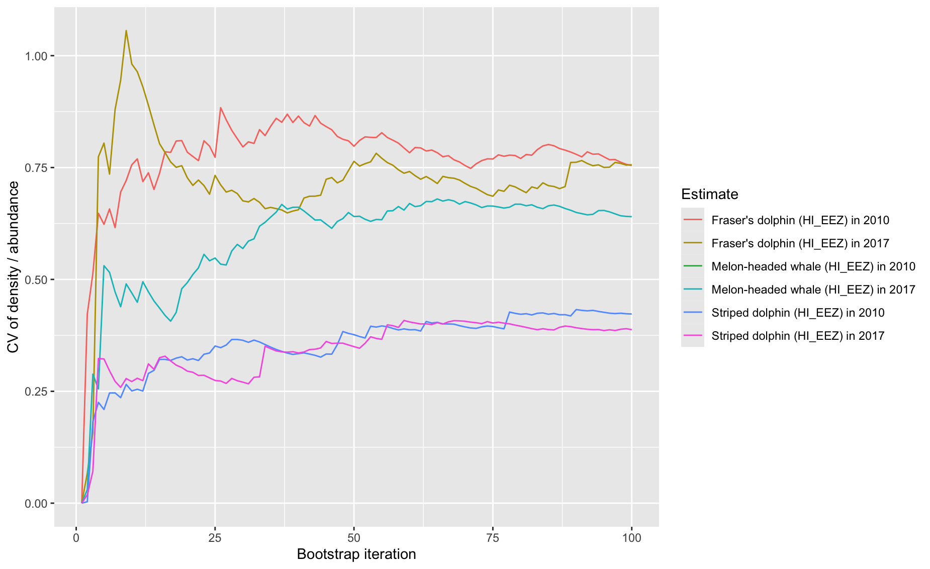
8 - Time series of point estimate CV as bootstraps accumulate
======================================================To call specific outputs and not others, use the options input. We demonstrate this be stepping through each output below.
Option 1: The point estimate
lta_diagnostics(lta_result, options = 1)
               title species   Region    Area year segments    km Area_covered
1    Striped dolphin     013 (HI_EEZ) 2474596 2010      124 17004        60114
2    Striped dolphin     013 (HI_EEZ) 2474596 2017      130 16281        57920
3   Fraser's dolphin     026 (HI_EEZ) 2474596 2010      124 17004        60611
4   Fraser's dolphin     026 (HI_EEZ) 2474596 2017      130 16281        48570
5 Melon-headed whale     031 (HI_EEZ) 2474596 2010      124 17004           NA
6 Melon-headed whale     031 (HI_EEZ) 2474596 2017      130 16281        54198
  ESW_mean  n g0_est ER_clusters D_clusters N_clusters size_mean size_sd     ER
1     3.54 19   0.33      0.0011     0.0005     1215.9      51.4    47.2 0.0574
2     3.56 17   0.32      0.0010     0.0005     1182.4      35.4    18.1 0.0369
3     3.56  3   0.33      0.0002     0.0001      186.4     236.2   129.0 0.0417
4     2.98  2   0.32      0.0001     0.0001      160.2     355.6    91.4 0.0437
5       NA  0   0.33      0.0000     0.0000        0.0        NA      NA 0.0000
6     3.33  3   0.32      0.0002     0.0001      214.8     189.2    68.4 0.0349
       D     N g0_small g0_large g0_cv_small g0_cv_large
1 0.0237 58531     0.33     0.33        0.20        0.20
2 0.0157 38919     0.32     0.32        0.21        0.21
3 0.0181 44761     0.33     0.33        0.20        0.20
4 0.0227 56161     0.32     0.32        0.21        0.21
5 0.0000     0     0.33     0.33        0.20        0.20
6 0.0162 39967     0.32     0.32        0.21        0.21
Option 2: Summary of bootstrap iterations
lta_diagnostics(lta_result, options = 2)
               title   Region year species iterations ESW_mean   g0_mean
1   Fraser's dolphin (HI_EEZ) 2010     026        100 3.674369 0.3348392
2   Fraser's dolphin (HI_EEZ) 2017     026        100 3.271689 0.3249818
3 Melon-headed whale (HI_EEZ) 2010     031        100      NaN 0.3348392
4 Melon-headed whale (HI_EEZ) 2017     031        100 3.099253 0.3249818
5    Striped dolphin (HI_EEZ) 2010     013        100 3.570792 0.3348392
6    Striped dolphin (HI_EEZ) 2017     013        100 3.603723 0.3249818
      g0_cv       km         ER          D      size    Nmean  Nmedian      Nsd
1 0.2189724 16942.74 0.03958147 0.01834906 227.12826 45406.50 36253.58 38049.74
2 0.2301472 16175.22 0.04336513 0.02214479 361.68608 54799.41 48096.98 43755.20
3 0.2189724 16942.74 0.00000000 0.00000000       NaN     0.00     0.00     0.00
4 0.2301472 16175.22 0.03765432 0.02099326 190.42373 51949.83 42732.64 36070.59
5 0.2189724 16942.74 0.05620828 0.02367771  51.00669 58592.76 55156.85 23004.54
6 0.2301472 16175.22 0.03370776 0.01498972  34.21571 37093.50 34313.40 14764.83
         CV      L95      U95
1 0.8379799 11351.63 181626.0
2 0.7984612 13699.85 219197.6
3       NaN      NaN      NaN
4 0.6943350 17316.61 155849.5
5 0.3926174 29296.38 117185.5
6 0.3980437 18546.75  74187.0
Option 3: Plot of detection function
Option 4: Histogram of bootstrapped detection counts
Option 5: Histogram of bootstrapped g(0) values
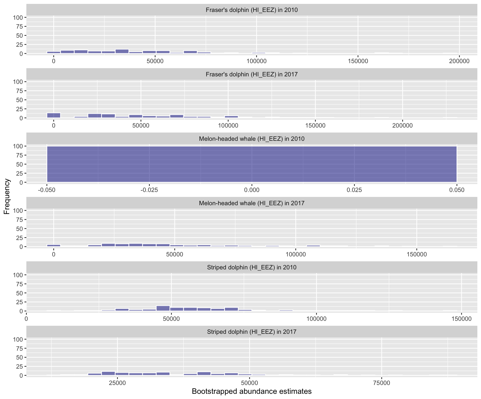
Option 6: Histogram of bootstrapped abundance estimates
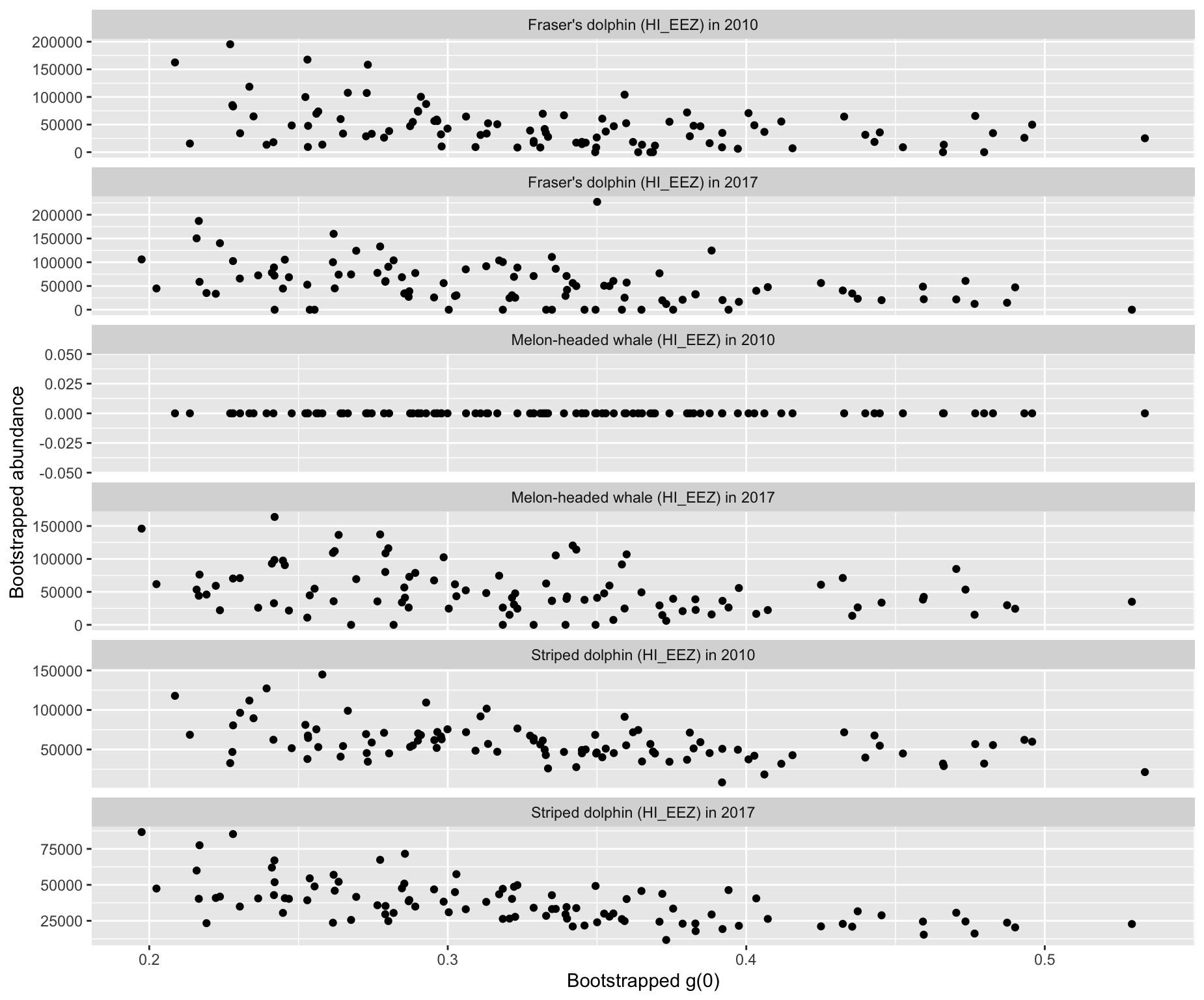
Option 7: Relationship between bootstrap g(0) and abudance
Option 8: Running calculation of CV during bootstrap process