Chapter 3 Data processing
In our WHICEAS case study example, we are interested in estimating density/abundance for 2017 and 2020 only, but we want to use surveys from previous years to help model species detection functions. We will therefore be using a dataset of NOAA Fisheries surveys in the Central North Pacific from 1986 to 2020.
To follow along, this data file can be downloaded here. (Right-click link and select “Save Link As…”.)
If they are not still in your work environment, you will need to load your saved settings compiled at the end of the vignette settings page:
You can process your survey data with these sightings using a single function, process_surveys(), which takes two primary arguments: the filepath(s) to your DAS survey data, and your settings object. For example:
That single command will convert your raw DAS data to a “cruz” object, a list of polished datasets that are prepared to be passed to subsequent analyses.
In our case we will use a third argument, edits, to apply edits to the DAS data before processing (see previous page for details on those edits) …
… and a fourth argument, seed, which controls random number generation in order to ensure the segments are chopped reproducibly:
Behind the scenes
The process_surveys() function is a wrapper for several discrete stages of data formatting/processing. Behind the scenes, each of those stages is carried out using a specific LTabundR function. The remainder of this page is a detailed step-by-step explanation of the data processing that occurs when you call process_surveys().
Edit cruise data
If the edits input argument is supplied to process_surveys(), temporary copies of the DAS file(s) are made and edited before processing. This step is discussed on the previous page and implemented with the function das_editor_tofile():
This function produces new DAS files with the edits applied, and returns an updated set of DAS filenames you can pass to the next stage of data processing.
Bring in cruise data
Read in and process your .DAS file using the functions in Sam Woodward’s swfscDAS package. To do so quickly, we built a wrapper function that makes this quick and easy:
Interpolate cruise data
Run the following function if you wish to interpolate the DAS data to a more frequent time interval, which can be useful for stratum assignment and effort calculations in some circumstances. This is only done in process_surveys() if the settings object passed to it has the interpolate input for load_survey_settings() set to a number (indicating the desired interval in seconds). In this example the interval is set to 120 seconds. Interpolation will only occur for On-Effort rows.
Note that this was just an example of how to use this feature.The dataset we carry forward from here will not be interpolated.
Process strata
Run the following function to add strata and study-area information to each row of DAS data:
This function loops through each stratum data.frame you have provided it in settings$strata, formats the stratum, and asks whether each DAS row occurs within it. For each stratum, a column named stratum_<StratumName> is added to the das object; each row in this column is TRUE (included) or FALSE.
Format DAS data into a cruz object
The function das_format() takes care of some final formatting and initiates the cruz object data structure.
This function (1) removes rows with invalid Cruise numbers, times, or locations; (ii) calculates the distance, in km, between each row of data; (iii) adds a ship column to the dataset, with initials for the ship corresponding to each cruise; (iv) creates a new list, cohorts, which copies the cruise data for each cohort specified in your settings; and (v) adds a stratum column to the data in each cohort. That column specifies
a single stratum assignment for each row of DAS data in the event of overlapping strata, based upon the cohort setting stratum_overlap_handling.
The cruz object
The function das_format() returns a list, which we have saved in an object named cruz, with several slots:
The slots strata and study_area provide the area, in square km, of each polygon being used:
cruz$strata
           stratum                area
1           HI_EEZ  2474595.762 [km^2]
2         OtherCNP 33817779.065 [km^2]
3              MHI   212033.063 [km^2]
4          WHICEAS   402948.734 [km^2]
5       Spotted_OU     5102.666 [km^2]
6       Spotted_FI    10509.869 [km^2]
7       Spotted_BI    39454.720 [km^2]
8  Bottlenose_KaNi     2755.024 [km^2]
9  Bottlenose_OUFI    14417.027 [km^2]
10   Bottlenose_BI     4668.072 [km^2]
11        nwhi_fkw   449375.569 [km^2]
12         mhi_fkw   171283.791 [km^2]
The slot cohorts is itself a list with one slot for each cohort. The slots are named using the id cohort setting.
Each cohort slot has a copy of the DAS data with a new stratum column, which contains a stratum assignment tailored to its cohort-specific settings. For instance, the all cohort, whose stratum_overlap_handling is set to "smallest", assigns the smallest stratum in the event of overlapping or nested strata:
Since the bottlenose cohort uses a different subset of geostrata, its distribution of stratum assignments will also differ:
cruz$cohorts$bottlenose$stratum %>% table(useNA='ifany')
.
  Bottlenose_BI Bottlenose_KaNi Bottlenose_OUFI          HI_EEZ        OtherCNP
           3415            1495            6862          117715          126252
        WHICEAS
          73899
This list, with these three primary slots, will be referred to from hereon as a cruz object.
Segmentize the data
To allocate survey data into discrete ‘effort segments’, which are used in variance estimation in subsequent steps, run the function segmentize(). This process is controlled by both survey-wide and cohort-specific settings, which are now carried in a slot within the cruz object. The process is outlined in detail in the Appendix on segmentizing.
This function does not change the high-level structure of the cruz object …
… or the cohort names in the cohorts slot:
For each cohorts slot, the list structure is the same:
cruz$cohorts$all %>% names
[1] "segments" "das"

cruz$cohorts$bottlenose %>% names
[1] "segments" "das"

cruz$cohorts$spotted %>% names
[1] "segments" "das"
The segments slot contains summary data for each effort segment, including start/mid/end coordinates, average conditions, and segment distance:
cruz$cohorts$all$segments %>% glimpse
Rows: 1,456
Columns: 39
$ seg_id       <dbl> 2051, 2062, 2055, 2063, 2064, 2056, 2065, 2066, 2067, 205…
$ Cruise       <dbl> 901, 901, 901, 901, 901, 901, 901, 901, 901, 901, 901, 90…
$ ship         <chr> "OES", "OES", "OES", "OES", "OES", "OES", "OES", "OES", "…
$ stratum      <chr> "WHICEAS", "WHICEAS", "WHICEAS", "WHICEAS", "WHICEAS", "W…
$ use          <lgl> FALSE, TRUE, TRUE, TRUE, TRUE, TRUE, TRUE, TRUE, TRUE, TR…
$ Mode         <chr> "C-P", "C", "C", "C-P", "P-C", "C", "C", "C", "C", "C", "…
$ EffType      <chr> "S", "S", "N", "S", "S", "N", "S", "S", "S", "N", "N", "N…
$ OnEffort     <lgl> TRUE, TRUE, TRUE, TRUE, TRUE, TRUE, TRUE, TRUE, TRUE, TRU…
$ ESWsides     <dbl> 2, 2, 2, 2, 2, 2, 2, 2, 2, 2, 2, 2, 2, 2, 2, 2, 2, 2, 2, …
$ dist         <dbl> 0.1224221, 145.5464171, 38.3219637, 148.8739186, 151.6705…
$ minutes      <dbl> 0.400, 515.450, 136.800, 540.017, 558.767, 40.900, 507.20…
$ n_rows       <int> 82, 188, 75, 178, 169, 31, 197, 146, 189, 51, 210, 63, 16…
$ min_line     <int> 424496, 424498, 424734, 424892, 425505, 425680, 425789, 4…
$ max_line     <int> 427047, 424891, 424831, 425504, 425788, 425735, 426303, 4…
$ year         <dbl> 2009, 2009, 2009, 2009, 2009, 2009, 2009, 2009, 2009, 200…
$ month        <dbl> 2, 2, 2, 2, 2, 2, 2, 2, 2, 2, 2, 2, 2, 2, 2, 2, 2, 2, 2, …
$ day          <int> 6, 6, 6, 7, 9, 10, 10, 11, 12, 12, 14, 15, 16, 16, 17, 18…
$ lat1         <dbl> 21.998167, 21.998167, 21.669333, 20.541000, 19.628833, 21…
$ lon1         <dbl> -159.1487, -159.1487, -158.0867, -157.5555, -156.2075, -1…
$ DateTime1    <dttm> 2009-02-06 07:33:52, 2009-02-06 07:33:52, 2009-02-06 15:…
$ timestamp1   <dbl> 1233905632, 1233905632, 1233932684, 1233999718, 123417162…
$ yday1        <dbl> 37, 37, 37, 38, 40, 41, 41, 42, 43, 43, 45, 46, 47, 47, 4…
$ lat2         <dbl> 19.193833, 20.541000, 21.591500, 19.621833, 21.143500, 21…
$ lon2         <dbl> -156.0575, -157.5555, -157.8283, -156.1827, -158.0830, -1…
$ DateTime2    <dttm> 2009-02-14 08:21:51, 2009-02-07 09:41:58, 2009-02-06 17:…
$ timestamp2   <dbl> 1234599711, 1233999718, 1233942729, 1234171624, 123426333…
$ yday2        <dbl> 45, 38, 37, 40, 41, 41, 42, 43, 45, 43, 46, 47, 47, 49, 4…
$ mlat         <dbl> 21.426500, 21.788500, 21.737833, 19.607500, 19.771167, 21…
$ mlon         <dbl> -158.9077, -158.5185, -157.9085, -156.1373, -156.8483, -1…
$ mDateTime    <dbl> 1234286319, 1233923429, 1233938494, 1234086957, 123418822…
$ mtimestamp   <dbl> 1234286319, 1233923429, 1233938494, 1234086957, 123418822…
$ avgBft       <dbl> NaN, 3.620949, 4.431633, 3.496502, 3.708160, 2.000000, 1.…
$ avgSwellHght <dbl> NaN, 3.740710, 4.000000, 2.663336, 3.062949, 2.000000, 2.…
$ avgHorizSun  <dbl> NaN, 4.758324, 4.073185, 4.842962, 8.780615, 9.000000, 5.…
$ avgVertSun   <dbl> NaN, 2.062058, 1.349072, 1.577954, 1.426446, 2.688592, 1.…
$ avgGlare     <dbl> NaN, 0.5453850, 0.0000000, 0.1182550, 0.1545467, 0.000000…
$ avgVis       <dbl> NaN, 6.750312, 6.176895, 6.483022, 5.771184, 6.500000, 6.…
$ avgCourse    <dbl> NaN, 106.2314, 113.4356, 208.8357, 288.5192, 205.4784, 21…
$ avgSpdKt     <dbl> NaN, 9.216194, 8.912595, 9.110399, 8.827567, 9.181559, 9.…
# Number of segments
cruz$cohorts$all$segments %>% nrow
[1] 1456
# Segment length distribution
x <- cruz$cohorts$all$segments$dist
hist(x,
breaks = seq(0,ceiling(max(x, na.rm=TRUE)),by=1),
xlab='Segment lengths (km)',
main=paste0('Target km: ',settings$survey$segment_target_km))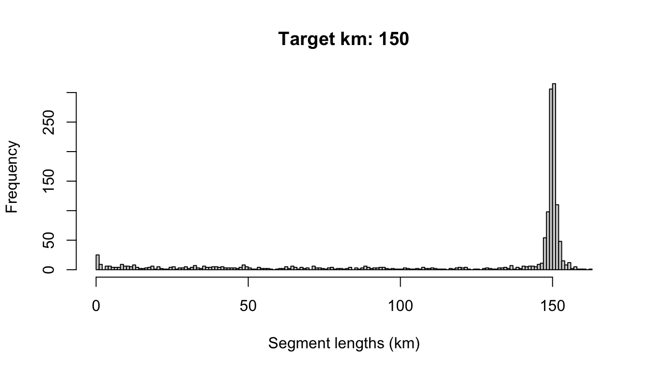
And the das slot holds the original data.frame of DAS data, modified slightly: the column OnEffort has been modified according to Beaufort range conditions, and the column seg_id indicates which segment the event occurs within.
cruz$cohorts$all$das %>% names
 [1] "Event"            "DateTime"         "Lat"              "Lon"
 [5] "OnEffort"         "Cruise"           "Mode"             "OffsetGMT"
 [9] "EffType"          "ESWsides"         "Course"           "SpdKt"
[13] "Bft"              "SwellHght"        "WindSpdKt"        "RainFog"
[17] "HorizSun"         "VertSun"          "Glare"            "Vis"
[21] "ObsL"             "Rec"              "ObsR"             "ObsInd"
[25] "Data1"            "Data2"            "Data3"            "Data4"
[29] "Data5"            "Data6"            "Data7"            "Data8"
[33] "Data9"            "Data10"           "Data11"           "Data12"
[37] "EffortDot"        "EventNum"         "file_das"         "line_num"
[41] "stratum_HI_EEZ"   "stratum_OtherCNP" "stratum_WHICEAS"  "year"
[45] "month"            "day"              "yday"             "km_valid"
[49] "km_int"           "km_cum"           "ship"             "stratum"
[53] "use"              "eff_bloc"         "seg_id"
The segmentize() function and its associated settings were designed to give researchers full control over how data are segmented, be it for design-based density analysis (which tend to use long segments of 100 km or more and allow for non-contiguous effort to be included in the same segment) or for habitat modeling (which tend to use short segments of 5 - 10 km and disallow non-contiguous effort to be pooled into the same segment). To demonstrate that versatility, checkout the Appendix on segmentizing.
Process sightings
To process sightings for each cohort of species, use the function process_sightings(). This function has three basic steps: for each cohort, the function (1) prepares a sightings table using the function das_sight() from swfscDAS; (2) filters those sightings to species codes specified for the cohort in your settings input; and (3) evaluates each of those sightings, asking if each should be included in the analysis according to your settings.
The function produces a formatted dataset and adds it to a new sightings slot.
cruz$cohorts$all %>% names
[1] "segments"  "das"       "sightings"

cruz$cohorts$bottlenose %>% names
[1] "segments"  "das"       "sightings"

cruz$cohorts$spotted %>% names
[1] "segments"  "das"       "sightings"
Note that the sightings table has a column named included (TRUE = yes, use it in the analysis). Any sightings that do not meet the inclusion criteria as specified in your settings will be included = FALSE, but they won’t be removed from the data.
The sightings table also has a new column, ss_valid,
indicating whether or not the group size estimate for this sighting
is valid and appropriate for use in abundance estimation and detection function fitting when group size is used as a covariate.
Since the sightings in each cohort are processed slightly differently according to the cohort’s specific settings – most importantly the species that will be included – you should expect different numbers of included/excluded sightings in each cohort dataset:
cruz$cohorts$all$sightings$included %>% table
.
FALSE  TRUE
  806  3128

cruz$cohorts$bottlenose$sightings$included %>% table
.
FALSE  TRUE
  113   410
When this function’s verbose argument is TRUE (the default), a message is printed each time a sighting does not meet the inclusion criteria.
Sightings data structure
The sightings table has many other variables:
cruz$cohorts$all$sightings %>% names
 [1] "Event"            "DateTime"         "Lat"              "Lon"
 [5] "OnEffort"         "Cruise"           "Mode"             "OffsetGMT"
 [9] "EffType"          "ESWsides"         "Course"           "SpdKt"
[13] "Bft"              "SwellHght"        "WindSpdKt"        "RainFog"
[17] "HorizSun"         "VertSun"          "Glare"            "Vis"
[21] "ObsL"             "Rec"              "ObsR"             "ObsInd"
[25] "EffortDot"        "EventNum"         "file_das"         "line_num"
[29] "stratum_HI_EEZ"   "stratum_OtherCNP" "stratum_WHICEAS"  "year"
[33] "month"            "day"              "yday"             "km_valid"
[37] "km_int"           "km_cum"           "ship"             "stratum"
[41] "use"              "eff_bloc"         "seg_id"           "SightNo"
[45] "Subgroup"         "SightNoDaily"     "Obs"              "ObsStd"
[49] "Bearing"          "Reticle"          "DistNm"           "Cue"
[53] "Method"           "Photos"           "Birds"            "CalibSchool"
[57] "PhotosAerial"     "Biopsy"           "CourseSchool"     "TurtleSp"
[61] "TurtleGs"         "TurtleJFR"        "TurtleAge"        "TurtleCapt"
[65] "PinnipedSp"       "PinnipedGs"       "BoatType"         "BoatGs"
[69] "PerpDistKm"       "species"          "best"             "low"
[73] "high"             "prob"             "mixed"            "ss_tot"
[77] "lnsstot"          "ss_percent"       "n_sp"             "n_obs"
[81] "n_best"           "n_low"            "n_high"           "calibr"
[85] "ss_valid"         "mixed_max"        "spp_max"          "included"
Columns 44 onwards correspond to sightings information. Columns of note:
speciescontains the species code. There is only one species-code per row (i.e, multi-species sightings have been expanded to multiple rows).best,low, andhighcontain the refined group size estimates, averaged across observers and calibrated according to the cohort’s settings specifications. For multi-species sightings, these numbers represent the number of individuals for the single species represented in the row (i.e., the original group size estimate has been scaled by the percentage attritbuted to this species).The columns following those group size estimates (
probthroughspp_max) detail how group sizes were estimated:probindicates whether probable species codes were accepted;mixedindicates whether this species’ sighting is part of a mixed-species sighting;n_spprovides the number of species occurring in this sighting;n_obsgives the number of observers who contributed group size estimates;n_bestthroughn_highgives the number of valid group size estimates given; andcalibrindicates whether or not calibration was applied to this sighting (based on the settings; see next section);mixed_maxindicates whether this species was the most abundant in the sighting (if multi-species);spp_maxindicates the species code for the most abundant species in the sighting (if multi-species). The columnss_validindicates whether or not sufficient data were available to produce a group size estimate usable in detection function model fitting and abundance estimation. For more details, see the “Missing data” paragraphs below.As explained above, the final column,
included, indicates whether this species should be included in the analysis.
Here is a glimpse of the data:
cruz$cohorts$all$sightings %>% glimpse
Rows: 3,934
Columns: 88
$ Event            <chr> "S", "S", "S", "S", "S", "S", "S", "S", "S", "S", "S"…
$ DateTime         <dttm> 2009-02-06 09:50:14, 2009-02-06 11:11:17, 2009-02-06…
$ Lat              <dbl> 21.93600, 21.83917, 21.78333, 21.70433, 21.69733, 21.…
$ Lon              <dbl> -158.8153, -158.6568, -158.4722, -158.2835, -158.2485…
$ OnEffort         <lgl> TRUE, TRUE, TRUE, TRUE, TRUE, TRUE, TRUE, TRUE, TRUE,…
$ Cruise           <dbl> 901, 901, 901, 901, 901, 901, 901, 901, 901, 901, 901…
$ Mode             <chr> "C", "C", "C", "C", "C", "C", "C", "C", "C", "C", "C"…
$ OffsetGMT        <int> 10, 10, 10, 10, 10, 10, 10, 10, 10, 10, 10, 10, 10, 1…
$ EffType          <chr> "S", "S", "S", "S", "S", "S", "S", "N", "N", "N", "N"…
$ ESWsides         <dbl> 2, 2, 2, 2, 2, 2, 2, 2, 2, 2, 2, 2, 2, 2, 2, 2, 2, 2,…
$ Course           <dbl> 167, 108, 111, 106, 106, 102, 102, 39, 39, 39, 39, 94…
$ SpdKt            <dbl> 9.4, 8.6, 9.2, 10.4, 10.4, 10.2, 10.2, 9.1, 9.1, 9.1,…
$ Bft              <dbl> 4, 4, 3, 2, 2, 2, 2, 3, 3, 3, 4, 4, 5, 5, 5, 5, 4, 2,…
$ SwellHght        <dbl> 4, 4, 4, 4, 4, 4, 4, 4, 4, 4, 4, 4, 4, 4, 4, 4, 3, 1,…
$ WindSpdKt        <dbl> 15, 11, 6, 3, 3, 4, 4, 9, 9, 9, 15, 15, 15, 17, 17, 1…
$ RainFog          <dbl> 1, 1, 1, 1, 1, 1, 1, 1, 1, 1, 1, 5, 5, 5, 5, 3, 1, 5,…
$ HorizSun         <dbl> 1, 2, 3, 3, 3, 4, 4, 4, 4, 4, 4, 5, 5, 5, 3, 3, 12, N…
$ VertSun          <dbl> 2, 2, 2, 1, 1, 1, 1, 1, 1, 1, 1, 1, 1, 1, 2, 2, 3, NA…
$ Glare            <lgl> TRUE, FALSE, FALSE, FALSE, FALSE, FALSE, FALSE, FALSE…
$ Vis              <dbl> 7.0, 7.0, 7.0, 7.0, 7.0, 7.0, 7.0, 7.0, 7.0, 7.0, 7.0…
$ ObsL             <chr> "197", "308", "086", "197", "197", "307", "307", "308…
$ Rec              <chr> "309", "307", "238", "309", "309", "197", "197", "307…
$ ObsR             <chr> "086", "197", "308", "086", "086", "309", "309", "197…
$ ObsInd           <chr> NA, NA, NA, NA, NA, NA, NA, NA, NA, NA, NA, NA, NA, N…
$ EffortDot        <lgl> TRUE, TRUE, TRUE, TRUE, TRUE, TRUE, TRUE, TRUE, TRUE,…
$ EventNum         <chr> "027", "061", "129", "168", "176", "188", "191", "204…
$ file_das         <chr> "CenPac1986-2020_Final_alb_edited_example.das", "CenP…
$ line_num         <int> 424551, 424585, 424655, 424696, 424704, 424716, 42471…
$ stratum_HI_EEZ   <lgl> TRUE, TRUE, TRUE, TRUE, TRUE, TRUE, TRUE, TRUE, TRUE,…
$ stratum_OtherCNP <lgl> TRUE, TRUE, TRUE, TRUE, TRUE, TRUE, TRUE, TRUE, TRUE,…
$ stratum_WHICEAS  <lgl> TRUE, TRUE, TRUE, TRUE, TRUE, TRUE, TRUE, TRUE, TRUE,…
$ year             <dbl> 2009, 2009, 2009, 2009, 2009, 2009, 2009, 2009, 2009,…
$ month            <dbl> 2, 2, 2, 2, 2, 2, 2, 2, 2, 2, 2, 2, 2, 2, 2, 2, 2, 2,…
$ day              <int> 6, 6, 6, 6, 6, 6, 6, 6, 6, 6, 6, 6, 6, 6, 6, 6, 7, 8,…
$ yday             <dbl> 37, 37, 37, 37, 37, 37, 37, 37, 37, 37, 37, 37, 37, 3…
$ km_valid         <lgl> TRUE, TRUE, TRUE, TRUE, TRUE, TRUE, TRUE, TRUE, TRUE,…
$ km_int           <dbl> 0, 0, 0, 0, 0, 0, 0, 0, 0, 0, 0, 0, 0, 0, 0, 0, 0, 0,…
$ km_cum           <dbl> 142323.0, 142344.5, 142366.8, 142388.5, 142392.2, 142…
$ ship             <chr> "OES", "OES", "OES", "OES", "OES", "OES", "OES", "OES…
$ stratum          <chr> "WHICEAS", "WHICEAS", "WHICEAS", "WHICEAS", "WHICEAS"…
$ use              <lgl> TRUE, TRUE, TRUE, TRUE, TRUE, TRUE, TRUE, TRUE, TRUE,…
$ eff_bloc         <chr> "291-0-0", "291-0-0", "291-0-0", "291-0-0", "291-0-0"…
$ seg_id           <dbl> 2062, 2062, 2062, 2062, 2062, 2062, 2062, 2055, 2055,…
$ SightNo          <chr> "001", "002", "003", "004", "005", "006", "007", "008…
$ Subgroup         <chr> NA, NA, NA, NA, NA, NA, NA, NA, NA, NA, NA, NA, NA, N…
$ SightNoDaily     <chr> "20090206_1", "20090206_2", "20090206_3", "20090206_4…
$ Obs              <chr> "086", "197", "308", "086", "086", "309", "307", "308…
$ ObsStd           <lgl> TRUE, TRUE, TRUE, TRUE, TRUE, TRUE, TRUE, TRUE, TRUE,…
$ Bearing          <dbl> 78, 3, 23, 5, 57, 49, 331, 354, 358, 7, 260, 42, 12, …
$ Reticle          <dbl> 1.4, 0.3, 2.0, 1.4, 1.0, 2.0, 0.8, 8.0, 0.1, NA, NA, …
$ DistNm           <dbl> 2.17, 4.10, 1.76, 2.17, 2.58, 1.76, 2.87, 0.31, 5.27,…
$ Cue              <dbl> 2, 6, 6, 3, 6, 6, 6, 6, 6, 6, 3, 6, 3, 6, 6, 6, 6, 6,…
$ Method           <dbl> 4, 4, 4, 4, 4, 4, 4, 4, 4, 1, 1, 4, 4, 4, 2, 4, 4, 4,…
$ Photos           <chr> "N", "N", "N", "N", "N", "N", "N", "N", "N", "N", "N"…
$ Birds            <chr> "N", "N", "N", "N", "N", "N", "N", "N", "N", "N", "N"…
$ CalibSchool      <chr> "N", "N", "N", "N", "N", "N", "N", "N", "N", "N", "N"…
$ PhotosAerial     <chr> "N", "N", "N", "N", "N", "N", "N", "N", "N", "N", "N"…
$ Biopsy           <chr> "Y", "N", "N", "N", "N", "N", "N", "N", "N", "N", "N"…
$ CourseSchool     <dbl> NA, NA, NA, NA, NA, NA, NA, NA, NA, NA, NA, NA, NA, N…
$ TurtleSp         <chr> NA, NA, NA, NA, NA, NA, NA, NA, NA, NA, NA, NA, NA, N…
$ TurtleGs         <dbl> NA, NA, NA, NA, NA, NA, NA, NA, NA, NA, NA, NA, NA, N…
$ TurtleJFR        <chr> NA, NA, NA, NA, NA, NA, NA, NA, NA, NA, NA, NA, NA, N…
$ TurtleAge        <chr> NA, NA, NA, NA, NA, NA, NA, NA, NA, NA, NA, NA, NA, N…
$ TurtleCapt       <chr> NA, NA, NA, NA, NA, NA, NA, NA, NA, NA, NA, NA, NA, N…
$ PinnipedSp       <chr> NA, NA, NA, NA, NA, NA, NA, NA, NA, NA, NA, NA, NA, N…
$ PinnipedGs       <dbl> NA, NA, NA, NA, NA, NA, NA, NA, NA, NA, NA, NA, NA, N…
$ BoatType         <chr> NA, NA, NA, NA, NA, NA, NA, NA, NA, NA, NA, NA, NA, N…
$ BoatGs           <dbl> NA, NA, NA, NA, NA, NA, NA, NA, NA, NA, NA, NA, NA, N…
$ PerpDistKm       <dbl> 3.9310187037330472925589, 0.3973973829439210736503, 1…
$ species          <chr> "076", "076", "076", "076", "076", "076", "076", "076…
$ best             <dbl> 1.000000, 2.057008, 1.030011, 1.986117, 1.000000, 1.1…
$ low              <dbl> 1.000000, 2.000000, 1.000000, 2.000000, 1.000000, 1.0…
$ high             <dbl> 1.000000, 3.000000, 1.246355, 2.000000, 2.000000, 1.0…
$ prob             <lgl> FALSE, FALSE, FALSE, FALSE, FALSE, FALSE, FALSE, FALS…
$ mixed            <lgl> FALSE, FALSE, FALSE, FALSE, FALSE, FALSE, FALSE, FALS…
$ ss_tot           <dbl> 1.000000, 2.057008, 1.030011, 1.986117, 1.000000, 1.1…
$ lnsstot          <dbl> 0.00000000, 0.72125271, 0.02956944, 0.68618171, 0.000…
$ ss_percent       <dbl> 1, 1, 1, 1, 1, 1, 1, 1, 1, 1, 1, 1, 1, 1, 1, 1, 1, 1,…
$ n_sp             <dbl> 1, 1, 1, 1, 1, 1, 1, 1, 1, 1, 1, 1, 1, 1, 1, 1, 1, 1,…
$ n_obs            <int> 1, 3, 3, 1, 1, 1, 1, 1, 2, 2, 1, 1, 1, 1, 1, 1, 2, 2,…
$ n_best           <int> 1, 3, 3, 1, 1, 1, 1, 1, 2, 2, 1, 1, 1, 1, 1, 1, 2, 2,…
$ n_low            <int> 1, 3, 3, 1, 1, 1, 1, 1, 2, 2, 1, 1, 1, 1, 1, 1, 2, 2,…
$ n_high           <int> 1, 3, 3, 1, 1, 1, 1, 1, 2, 2, 1, 1, 1, 1, 1, 1, 2, 2,…
$ calibr           <lgl> TRUE, TRUE, TRUE, TRUE, TRUE, TRUE, TRUE, TRUE, TRUE,…
$ ss_valid         <lgl> TRUE, TRUE, TRUE, TRUE, TRUE, TRUE, TRUE, TRUE, TRUE,…
$ mixed_max        <lgl> TRUE, TRUE, TRUE, TRUE, TRUE, TRUE, TRUE, TRUE, TRUE,…
$ spp_max          <chr> "076", "076", "076", "076", "076", "076", "076", "076…
$ included         <lgl> TRUE, TRUE, TRUE, TRUE, TRUE, TRUE, TRUE, TRUE, TRUE,…
Note that the process_sightings() function draws upon cruz$settings for inclusion criteria, but some of those settings can be overridden with the function’s manual inputs if you want to explore your options (see below).
Group size estimates
Group size calibration: In the settings we are using in this tutorial, group size estimates are adjusted using the calibration models from Barlow et al. (1998) (their analysis is refined slightly and further explained in Gerrodette et al. (2002)). These calibration corrections are observer-specific. Most observers tend to underestimate group size and their estimates are adjusted up; others tend to overestimate and their estimates are adjusted down. Some observers do not have calibration coefficients, and for them a generic adjustment (upwards, by dividing estimates by 0.8625) is used. Note that only the best estimates of size are calibrated; the high and low estimates are not.
Mean estimates across observers: In LTabundR, each observer’s estimate is calibrated, then all observer estimates are averaged. To do that averaging, our settings specify that we shall use a geometric mean, instead of an arithmetic mean. Since calibration is carried out, the geometric weighted mean is used, which weights school size estimates from multiple observers according to the variance of their calibration coefficients. (The weighted mean is used for high and low estimates as well, even though they are not calibrated, using the variance of the calibrated best estimates as weights.) When calibration is not carried out, the geometric unweighted mean is used for the best, high and low estimates.
Here are our current best estimates of group size:
cruz$cohorts$all$sightings$best %>% head(20)
 [1]   1.000000   2.057008   1.030011   1.986117   1.000000   1.159420
 [7]   2.318841   2.318841   3.666409   7.513902   2.783748   9.275362
[13]   3.478261   1.159420   1.986117   1.159420   1.000000   3.279336
[19]   8.115942 393.320601
# Verify that these estimates were calibrated
cruz$cohorts$all$sightings$calibr %>% head(20)
[1] TRUE TRUE TRUE TRUE TRUE TRUE TRUE TRUE TRUE TRUE TRUE TRUE TRUE TRUE TRUE
[16] TRUE TRUE TRUE TRUE TRUELet’s compare those estimates to unadjusted ones, in which calibration (and therefore weighted geometric mean) is turned off:
cruz_demo$cohorts$all$sightings$best %>% head(20)
 [1]   1.000000   2.000000   1.000000   2.000000   1.000000   1.000000
 [7]   2.000000   2.000000   3.162278   6.480741   3.000000   8.000000
[13]   3.000000   1.000000   2.000000   1.000000   1.000000   2.828427
[19]   7.000000 234.627970
# Verify that these estimates were *not* calibrated
cruz_demo$cohorts$all$sightings$calibr %>% head(20)
[1] FALSE FALSE FALSE FALSE FALSE FALSE FALSE FALSE FALSE FALSE FALSE FALSE
[13] FALSE FALSE FALSE FALSE FALSE FALSE FALSE FALSEYou can also carry out calibration corrections without using a geometric mean (the arithmetic mean will be used instead):
cruz_demo$cohorts$all$sightings$best %>% head(20)
 [1]   1.000000   2.166746   1.053140   1.986117   1.000000   1.159420
 [7]   2.318841   2.318841   4.057971   7.536232   2.783748   9.275362
[13]   3.478261   1.159420   1.986117   1.159420   1.000000   3.478261
[19]   8.115942 465.411665
# Verify that these estimates were indeed calibrated
cruz_demo$cohorts$all$sightings$calibr %>% head(20)
[1] TRUE TRUE TRUE TRUE TRUE TRUE TRUE TRUE TRUE TRUE TRUE TRUE TRUE TRUE TRUE
[16] TRUE TRUE TRUE TRUE TRUENote that when geometric_mean = TRUE but calibration is not carried out, the simple unweighted geometric mean is calculated instead of the weighted geometric mean, since the weights are the variance estimates from the calibration routine.
Also note that group size calibration is only carried out if the settings school_size_calibrate is TRUE and group_size_coefficients is not NULL. However, even when calibration coefficients are provided, it is possible to specify that calibration should only be carried out for raw estimates above a minimum threshold (see cohort setting calibration_floor, whose default is 0), since observers may be unlikely to mis-estimate the group size of a lone whale or pair. For observers who have calibration coefficients in the settings$group_size_coefficients table, that minimum is specified for each observer individually. For observers not in that table, calibration will only be applied to raw group size estimates above the settings$cohorts[[i]]$calibration_floor.
Missing data: Some sightings may be missing data regarding group size estimates: perhaps not all observers provided all three estimates (best-low-high), or perhaps not all observers provided group size percentages for mixed-species groups. When data are processed in LTabundR, the resulting sightings table includes a column, ss_valid, to indicate whether enough data were available to produce a group size estimate that is usable for detection function fitting and abundance estimation. The procedure for determining whether ss_valid is TRUE or FALSE for a sighting is as follows:
For each sighting, loop through each’s observer’s estimate of group size:
(Optional) Apply a calibration adjustment to the observer’s best estimate, as discussed above; if any part of the calibration adjustment process fails, the original estimates are used (observer’s
ss_validis stillTRUEfor the sighting).If the observer’s best estimate is
NAor less than0, the low estimate is used as the best estimate and the observer’sss_validbecomesFALSE.If the low estimate is
NAor less than0, the best estimate is coerced to1and the observer’sss_validremainsFALSE.After all observer estimates have been processed, filter to estimates where observer
ss_validisTRUE. If at least one observer estimate remains, the sighting’s overallss_validstatus isTRUE; if no estimates remain, the overallss_validstatus becomesFALSEand the best size estimate becomesNA.If
ss_validisTRUEafter this filter, the remaining observer estimates are used to find the geometric mean (or geometric weighted mean) estimate of group size. If that mean estimate is less than0orNAfor any reason, overallss_validbecomesFALSEand the geometric (weighted) mean of the raw low estimates is used. If the low estimate has to be used and it is less than0orNA, the best estimate becomes1and overallss_validremainsFALSE.For mixed-species groups: If multiple percentage estimates are available for a species in a mixed-species group, the average of those percentage estimates will be used (as discussed above). If only a single percentage estimate is available for a species in a mixed-species group, that single percentage estimate will be used (
ss_validwill not be changed). If no percentage estimate is available for a species in a mixed-species group, then the best estimate for that species will becomeNAandss_validwill becomeFALSEif it is not already.
Process subgroups
After sightings data are processed, the process_surveys() function calls the subroutine process_subgroups() to find and calculate subgroup group size estimates for false killer whales (or other species that may have been recorded using the subgroup functionality in WinCruz), if any occur in the DAS data (Event code “G”).
If subgroups are found, a subgroups slot is added to the analysis list for a cohort.
This subgroups slot holds a list with three dataframes:
$events(each row is a group size estimate for a single subgroup during a single phase of the false killer whale protocol (if applicable) within a single sighting; this is effectively the raw data). Internally,LTabundRuses the functionsubgroup_events()to produce thisdata.frame.$subgroups(each row is a single subgroup for a single protocol phase, with all group size estimates averaged together (both arithmetically and geometrically). Internally,LTabundRuses the functionsubgroup_subgroups()to produce thisdata.frame.$sightings(each row is a “group” size estimate for a single sighting during a single phase protocol, with all subgroup group sizes summed together). Note for false killer whales this “group” size estimate is not likely to represent actual group size because groups can be spread out over tens of kilometers, and it is not expected that every subgroup is detected during each protocol phase. Internally,LTabundRuses the functionsubgroup_sightings()to produce thisdata.frame.
For a detailed example of how subgroup data are analyzed, see the vignette page on subgroup analysis using data on Central North Pacific false killer whales.
Editing subgroup details
The subgroup protocol involves a few components that may not be adequately included in the raw DAS data, such as the assignment of subgroup detections to certain “phases” of the protocol or certain populations (or multiple populations). These details are described in detail on the vignette page on subgroup analysis, as is the process for manually updating the processed cruz object with those details. LTabundR includes several functions that facilitate this work.
Review
By the end of this process, you have a single data object, cruz, with all the data you need to move forward into the next stages of mapping and analysis.
The LTabundR function cruz_structure() provides a synopsis of the data structure:
cruz_structure(cruz)
"cruz" list structure ========================

$settings
         $strata --- with 12 polygon coordinate sets
         $survey --- with 16 input arguments
         $cohorts --- with 3 cohorts specified, each with 19 input arguments

$strata
       ... containing a summary dataframe of 12 geostrata and their spatial areas
       ... geostratum names:
           HI_EEZ, OtherCNP, MHI, WHICEAS, Spotted_OU, Spotted_FI, Spotted_BI, Bottlenose_KaNi, Bottlenose_OUFI, Bottlenose_BI, nwhi_fkw, mhi_fkw

$cohorts

        $all
            geostrata: WHICEAS, HI_EEZ, OtherCNP
            $segments  --- with 1454 segments (median = 149.4 km)
            $das       --- with 329638 data rows
            $sightings --- with 3934 detections
            $subgroups --- with 255 subgroups, 61 sightings, and 389 events

        $bottlenose
            geostrata: WHICEAS, HI_EEZ, OtherCNP, Bottlenose_BI, Bottlenose_OUFI, Bottlenose_KaNi
            $segments  --- with 1537 segments (median = 149.3 km)
            $das       --- with 329638 data rows
            $sightings --- with 523 detections

        $spotted
            geostrata: WHICEAS, HI_EEZ, OtherCNP, Spotted_OU, Spotted_FI, Spotted_BI
            $segments  --- with 1540 segments (median = 149.2 km)
            $das       --- with 329638 data rows
            $sightings --- with 527 detections
Each species-specific cohort has its own list under cruz$cohorts, and each of these cohorts has the same list structure:
segmentsis a summary table of segments.dasis the rawDASdata, modified withseg_idto associate each row with a segment.sightingsis a dataframe of sightings processed according to this cohort’s settings.subgroups(if any subgroup data exist in your survey) is a list with subgroup details.
In each cohort data.frame, there are three critically important columns to keep in mind:
seg_id: this column is used to indicate the segment ID that a row of data belongs to.use: this column indicates whether a row of effort should be used in the line-transect analysis. Every row of data within a single segment will have the sameusevalue.included: this column occurs in thesightingsdataframe only. It indicates whether the sightings should be included in line-transect analysis based on the specified settings. Any sighting withuse == FALSEwill also haveincluded == FALSE, but it is possible for sightings to haveuse == TRUEwithincluded == FALSE. For example, if the settingabeam_sightingsis set toFALSE, a sighting with a bearing angle beyond the ship’s beam can be excluded from the analysis (included == FALSE) even though the effort segment it occurs within will still be used (use == TRUE).
Finally, let’s save this cruz object locally, to use in downstream scripts: