Chapter 7 Estimating g(0)
Detection function models assume g(0) is 1.0.
In distance sampling, a “detection function” is fit to the perpendicular sighting distances to reflect the fact that animals farther out are more difficult to detect. That detection function is a model of how the probability of detection declines with increasing distance from your survey trackline. The equations for detection function models are all constructed to assume that the probability of detecting an animal on your trackline (distance = 0 km) is 1.0 – you never miss an animal on your trackline. This trackline detection probability is referred to as g(0).
In reality, though, it almost never is – and it greatly impacts results.
When searching for marine mammals at sea, even some of those occurring directly on your survey trackline will be missed. Real g(0) is actually less than 1.0. This technicality makes a big difference: if g(0) is actually 0.5, the assumption that g(0) is 1.0 will underestimate animal abundance by 50%. Some animals, such as pygmy and dwarf sperm whales (Kogia spp.), are very cryptic deep divers and easily missed or unavailable, and thus likely have a true g(0) below 0.1. This means that estimates assuming their g(0) is still 1.0 will underestimate true abundance by 90%! Moreover, all species – whether you are a pygmy sperm whale or a blue whale – become easier to miss when sighting conditions deteriorate (e.g., Beaufort sea states 4 - 6).
Therefore, g(0) must be estimated and then used to scale the detection function.
So g(0) matters, and the assumption of detection functions that g(0) = 1.0 is nearly always wrong. Luckily, there is a way to handle this that avoids constructing new detection function equations or estimating even more parameters during the detection function fitting process: we use an estimate of g(0) to scale the detection function. Say the detection function predicts that the probability of detection is 1.0, 0.8, and 0.6 at distances 0 km, 1 km, and 2km, respectively. If g(0) is actually 0.5, then we can scale the detection function so that those respective predictions are now 0.5, 0.4, and 0.3.
Estimating g(0) for a NOAA Fisheries line-transect cetacean survey generally involves four steps (Barlow 2015):
First, you estimate g(0) in “perfect” conditions (e.g., Beaufort sea state 0) to account for animal availability.
Second, you scale that estimate downward to approximate g(0) when conditions are less than ideal (i.e., a separate g(0) estimate for each Beaufort sea state from 1 to 6). This is known as the relative trackline detection probability, or relative g(0), or most simply: Rg(0).
Third, you determine the weighted average value of g(0) for your particular survey, based on the proportional distribution of effort in each sea state. You pass this single value to your line-transect analysis functions.
Fourth, you need to determine the CV of your weighted estimate of g(0). This isn’t straightforward, because you first need to simulate a new distribution for the weighted g(0) estimate, from which you then calculate the CV.
The first of these steps is typically the biggest lift analytically, and very few studies provide absolute estimates of g(0) for their species of interest. Doing so involves simulation modeling and specialized field methods (e.g., Barlow 1999).
Instead, most NOAA Fisheries studies assume that the absolute g(0) is in fact 1.0 – even though it’s not – and proceed directly to the second step – relative trackline detection probability, Rg(0). This is more common because it can be estimated directly from the survey data, thanks to an approach developed in Barlow (2015): “Inferring trackline detection probabilities, g(0), for cetaceans from apparent densities in different survey conditions”.
Relative g(0)
Archived Rg(0) estimates
As of 2022, most eastern and central Pacific NOAA Fisheries studies use the Rg(0) estimates from Barlow (2015), which are based on NOAA Fisheries cruises in the eastern and central Pacific from 1986 to 2010. LTabundR includes Barlow’s results in a built-in dataset.
Here is the top of this dataset, in which each row is a Rg(0) estimate for a single species - Beaufort sea state scenario.
barlow_2015 %>% head(12)
                    title             scientific             spp truncation
1           Delphinus spp              Delphinus     005-016-017        5.5
2           Delphinus spp              Delphinus     005-016-017        5.5
3           Delphinus spp              Delphinus     005-016-017        5.5
4           Delphinus spp              Delphinus     005-016-017        5.5
5           Delphinus spp              Delphinus     005-016-017        5.5
6           Delphinus spp              Delphinus     005-016-017        5.5
7           Delphinus spp              Delphinus     005-016-017        5.5
8  Stenella attenuata ssp Stenella attenuata ssp 002-006-089-090        5.5
9  Stenella attenuata ssp Stenella attenuata ssp 002-006-089-090        5.5
10 Stenella attenuata ssp Stenella attenuata ssp 002-006-089-090        5.5
11 Stenella attenuata ssp Stenella attenuata ssp 002-006-089-090        5.5
12 Stenella attenuata ssp Stenella attenuata ssp 002-006-089-090        5.5
   pooling regions bft   Rg0 Rg0_CV
1        1    none   0 1.000   0.00
2        1    none   1 1.000   0.00
3        1    none   2 0.940   0.25
4        1    none   3 0.722   0.25
5        1    none   4 0.485   0.14
6        1    none   5 0.394   0.20
7        1    none   6 0.404   0.50
8     none    none   0 1.000   0.00
9     none    none   1 0.728   0.03
10    none    none   2 0.531   0.06
11    none    none   3 0.386   0.09
12    none    none   4 0.282   0.12
This dataset includes Rg(0) estimates for the following species:
barlow_2015$title %>% unique
 [1] "Delphinus spp"               "Stenella attenuata ssp"
 [3] "Stenella longirostris ssp"   "Striped dolphin"
 [5] "Rough-toothed dolphin"       "Bottlenose dolphin"
 [7] "Risso's dolphin"             "Short-finned pilot whale"
 [9] "Killer whale"                "Sperm whale"
[11] "Kogia spp"                   "Cuvier's beaked whale"
[13] "Mesoplodon spp"              "Dall's porpoise"
[15] "Minke whale"                 "Sei/Bryde's"
[17] "Fin whale"                   "Blue whale"
[19] "Humpback whale"              "Unidentified dolphin"
[21] "Unidentified cetacean"       "Pacific white-sided dolphin"
[23] "Pygmy killer whale"          "False killer whale"
If your study species – or one with similar detectability – can be found on this list, then you can consider using this data.frame of Rg(0) values and moving on to the next step, especially if your survey was conducted in the eastern or Central Pacific.
Note that if you do not have a large survey dataset, this may be the only option available to you. Estimating new Rg(0) values requires a large number of sightings (i.e., hundreds) across many Beaufort states.
New Rg(0) estimates
LTabundR includes a function, g0_model(), which you can use to apply the Barlow (2015) modeling methods to generate new estimates of Rg(0) based on your own survey data or by combining your data with those used in the Barlow (2015) estimation.
To do this, you first need a cruz object in which effort has been split into short segments (5 - 10 km). If you want to work with NOAA Fisheries DAS data from the eastern and central Pacific, you can use a built-in dataset of 1986 - 2020 surveys that is processed specifically for use in Rg(0) estimation:
To use this dataset in R(0) estimation, we first filter it to systematic effort within sea states 0 - 6:
cruzi <- filter_cruz(noaa_10km_1986_2020,
                     analysis_only = TRUE,
                     eff_types = 'S',
                     bft_range = 0:6,
                     on_off = TRUE)
You can then estimate Rg(0) for each Beaufort sea state using the function g0_model(). For example, the code for striped dolphin (Stenella coeruleoalba) is as follows:
rg0 <- g0_model(spp = '013',
                truncation_distance = 5.5,
                cruz = cruzi,
                constrain_shape = TRUE,
                jackknife_fraction = .1,
                seed = 123)
The jackknife_fraction input indicates that the standard error and CV will be estimated using an iterative jackknife procedure in which 10% of the data is removed in each iteration. Find more details on this process using the function documentation, ?g0_model(). The seed input makes the jacknife process reproducible. It is optional and can be ignored or left NULL if you wish.
The input constrain_shape provides a way to ensure that the Rg(0) curve declines monotonically. Some modeled Rg(0) curves are liable to erreneously increase with increasing Bft due to low sample sizea at the lowest Bft (0-2) or highest Bft (5-6) states. To coerce monotonic decline, set this to TRUE, and the function will use a shape-constrained GAM (scam() from package scam) instead of a classic mgcv::gam(). We recommend beginning with NULL then modifying this if needed, based on the output: if the Rg(0) curve increases at any Bft state, try running again with constrain_shape set to TRUE. Note that this is an updated approach to the Bft-pooling method used in Barlow (2015).
The chief result of this function is a $summary table:
rg0$summary
  bft       Rg0      ESW  n     Rg0_SE     Rg0_CV     ESW_SE
1   0 1.0000000 3.830721 10 0.00000000 0.00000000 0.29802746
2   1 0.7042927 3.615397 10 0.01796678 0.02551039 0.23022945
3   2 0.4960188 3.381583 10 0.02523563 0.05087636 0.14893271
4   3 0.3493328 3.138417 10 0.02658750 0.07610937 0.07325895
5   4 0.2460263 2.894303 10 0.02490295 0.10122068 0.08049577
6   5 0.1732724 2.657071 10 0.02187068 0.12622140 0.15621342
7   6 0.1220358 2.436275 10 0.01844235 0.15112247 0.23037913
The model predicts that Rg(0) declines rapidly with deteriorating sea state:
plot(Rg0 ~ bft, data = rg0$summary,
     ylim=c(0,1), type='o', pch=16)
abline(h=seq(0,1,by=.1),
       col='grey85', lty=3)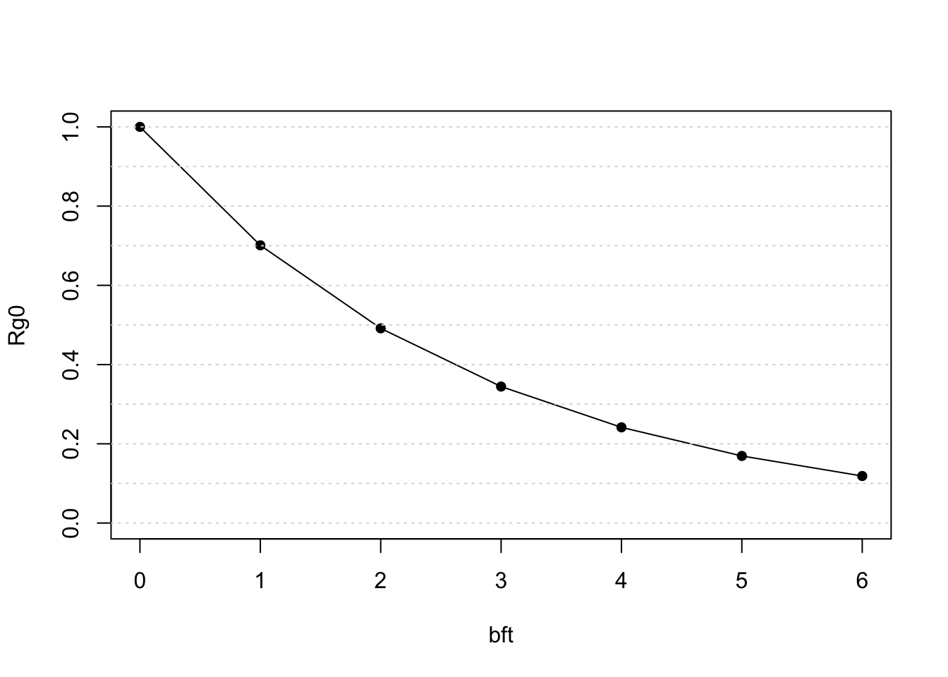
In addition to the summary above, this function returns various details, including the details of the Generalized Additive Model (GAM) (for both the estimate and the jackknifed datasets), and the raw sightings and segments used in the model.
To produce these estimates efficiently for many species, you can use the wrapper function g0_table(), as follows. First you build a list of parameters for each species/species group:
species <- list(
  list(spp = c('005', '016', '017'),
       title = 'Delphinus spp',
       constrain_shape = TRUE,
       truncation = 5.5),
  list(spp = '021',
       title = "Risso's dolphin",
       truncation = 5.5,
       constrain_shape = TRUE),
  list(spp = '046',
       title = 'Sperm whale',
       truncation = 5.5),
  list(spp = c('047', '048', '080'),
       title = 'Kogia spp',
       truncation = 4.0,
       constrain_shape = FALSE),
  list(spp = '061',
       title = "Cuvier's beaked whale",
       constrain_shape = TRUE,
       truncation = 4.0),
  list(spp = '074',
       title = 'Fin whale',
       truncation = 5.5,
       regions = 'CCS'))
Note that we used shorter truncation distances for cryptic species.
Note also that we had to pool Beaufort sea states 0-2 for Risso’s dolphins in order to maintain a monotonic decline in the Rg(0) ~ Beaufort curve.
Note also that we limited the geostrata used to model the fin whale Rg(0) curve to the California Current System (‘CCS’, after Barlow 2015), so that zero-inflated segments did not confound the model. In general we recommend that survey effort should only be included for regions within a species’ normal expected range. Otherwise zero-inflation may have an effect on Rg(0) model results.
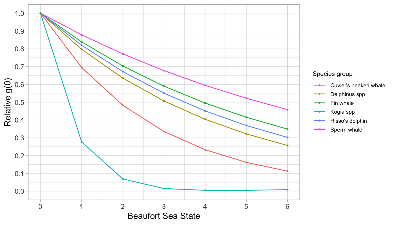
We then pass this species list to g0_table(). In this example, we are only estimating the Rg(0) relationship, without conducting jackknife estimation:
Now plot the result using a dedicated LTabundR function:
Weighted average g(0)
Since g(0) clearly depends upon survey conditions, and since each survey is carried out in a specific sequence of conditions, a unique, weighted g(0) value must be estimated for each species in each geostratum and survey of interest.
This will be done automatically by the line-transect analysis functions coming up (see LTabundR::lta()), meaning you only need a table of Rg(0) values in order to proceed to the next step. But you can also calculate weighted g(0) values separately as an isolated analysis, which we show below.
Let’s say we want to estimate the average g(0) for striped dolphins in the WHICEAS study area during the survey years of 2017 and 2020. From above, we have an estimate of the Rg(0) and its CV for each Beaufort state:
rg0$summary %>% select(bft, Rg0, Rg0_CV)
  bft       Rg0     Rg0_CV
1   0 1.0000000 0.00000000
2   1 0.7042927 0.02551039
3   2 0.4960188 0.05087636
4   3 0.3493328 0.07610937
5   4 0.2460263 0.10122068
6   5 0.1732724 0.12622140
7   6 0.1220358 0.15112247
We also have a processed cruz object with 2017 data:
To view the distribution of effort in this WHICEAS 2017 across sea states, we can use the function summarize_bft():
summarize_bft(cruz_17)$overall
# A tibble: 6 × 3
    Bft    km   prop
  <dbl> <dbl>  <dbl>
1     1  132. 0.0203
2     2  585. 0.0899
3     3  920. 0.141
4     4 2143. 0.329
5     5 1875. 0.288
6     6  853. 0.131
We then use the function g0_weighted_var() to compute the weighted Rg(0) for our survey as well as its CV. This function carries out an automated optimization routine to simulate a new distribution for the weighted g(0), which is then used to estimate the weighted CV.
weighted_g0_2017 <-
  g0_weighted(Rg0 = rg0$summary$Rg0,
              Rg0_cv = rg0$summary$Rg0_CV,
              cruz = cruz_17,
              seed = 123) # optional for reproducibility
The result:
Now let’s do the same for WHICEAS 2020 and compare the weighted g(0) estimate:
# Filter to 2020
cruz_20 <- filter_cruz(cruz_1720, years = 2020, verbose=FALSE)

# Summarize Bft effort
summarize_bft(cruz_20)$overall
# A tibble: 6 × 3
    Bft     km   prop
  <dbl>  <dbl>  <dbl>
1     1   84.3 0.0160
2     2  266.  0.0505
3     3  440.  0.0838
4     4 1458.  0.277
5     5 1968.  0.374
6     6 1042.  0.198
Note that conditions were a bit worse in 2020 compared to 2017. We therefore expect the weighted g(0) estimate to be lower:
weighted_g0_2020 <-
  g0_weighted(Rg0 = rg0$summary$Rg0,
              Rg0_cv = rg0$summary$Rg0_CV,
              cruz = cruz_20,
              seed = 123) # optional for reproducibility
The result:
Confirmed: weighted g(0) in the WHICEAS study area in 2020 is slightly lower than in 2017, due to generally worse survey conditions. These year-specific estimates should prevent those different conditions from impacting their respective abundance estimates.